install.packages("foo")2 Getting Started
2.1 Getting Started with R
TL;DR What you Need
To work with R in this course, you need to be able to run R code, mix it with prose and formulas in a notebook-style environment, and turn program and output into pdf and html files. To accomplish this you will need
R. Download from CRANRStudio. Download RStudio Desktop from Posit
LaTex. TinyTeX is a small distribution based on Tex Live that works well with
Rand can be manipulated through thetinytexRpackage.
You can skip R and RStudio installs if you do the work in a Posit Cloud account. These are available for free here.
To get started with R as a statistical programming language you need access to R itself and a development environment from which to submit R code.
Download R for your operating system from the CRAN site. CRAN is the “Comprehensive R Archive Network” and also serves as the package management system to add new packages to your installation.
If you use VS Code as a development environment, add the “R Extension for Visual Studio” to your environment. We are focusing on RStudio as a development environment here.
Posit Cloud
In today’s cloud world, you can get both through Posit Cloud. Posit is the company behind RStudio, Quarto, and other cool tools. Their cloud offering gives you access to an RStudio instance in the cloud. You can sign up for a free account here. The only drawback of the free account is its limitations in terms of RAM, CPU, execution time, etc. For the work you will be doing in this course, and probably many other courses, you will not exceed the limitations of the free account.
Once you have created an account, the workspace is organized the same way as a RStudio session on your desktop.
R and RStudio
RStudio is an integrated development environment (IDE) for R, but supports other languages as well. For example, using Quarto in RStudio, you can mix R, Python, and other code within the same document. Download Rstudio Desktop here.
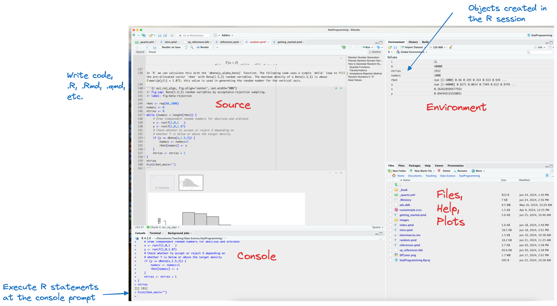
The RStudio IDE is organized in panes, each pane can have multiple tabs (Figure 2.1). The important panes are
Source. The files you edit. These can be R files (.R), Rmarkdown (.Rmd), Quarto (.qmd), or any other text files.
Console. Here you can enter
Rcommands directly at the command prompt “>”. This pane also has aTerminaltab for an OS terminal and aBackground Jobstab. The latter is important when you knit documents into pdf or html format.Envitonment. Displays information about the objects created in the
Rsession. You can click on an object for a more detailed look at it in theViewer.Help. This pane contains many useful tabs, such as a File browse, package information, access to the documentation and help system. Plots generated from the
Consoleor from anRscript are displayed in thePlotstab of this pane.
Package Management
The R installation comes with attached base packages, you do not need to install or load those. Any other packages are enabled in a two-step process:
- Install the package
- Load the package in your
Rsession with thelibrary()command.
Installing the package is done once, this step adds the package to your system. Loading the library associated with the package needs to be done in every R session. Without loading the library, R cannot find the functions exported by the library.
Installing standard packages
A standard R package is made available through the CRAN (Comprehensive R Archive Network) repositories. To install package “foo” from CRAN use
To install multiple packages, specify them as a character vector:
install.packages(c("foo","bar","foobar"))To uninstall (remove) one or more packages from a system, use the
remove.packages(c("foo","bar"))command.
Packages are installed by default into the directory given as the first element of the .libPaths() function. On my Mac this is
.libPaths()[1][1] "/Users/olivers/Library/R/arm64/4.4/library"If you wish to install a package in a different location, provide the location in the lib="" argument of install.packages(). Note that if you use a non-default location for the package install you need to specify that location when you load the library with the library command.
To make the functionality in a package available to your R session, use the library command. For example, the following statements make the dplyr and Rfast functions available.
library("dplyr")
library("Rfast")
Libraries export functions into the R name space and sometimes these can collide. For example, the Rfast package exports functions knn and knn.cv for \(k\)-nearest neighbor and cross-validated \(k\)-nearest neighbor analysis. Functions by the same name also exist in the class package. To make it explicit which function to use, prepend the function name with the package name:
Rfast::knn()

class::knn.cv()
To load a library from a non-standard location, for example, when you installed the package in a special directory by using lib= on install.packages(), you need to specify the lib.loc="" option in the library command.
install.packages("some_package_name", lib="/custom_path/to/packages/")

library("some_package_name", lib.loc="/custom_path/to/packages/")
All available packages in your R environment can be seen with the
library() command.
Libraries have dependencies and if you want to install all libraries that a given one depends on, choose dependencies=TRUE in the install.packages() call:
install.packages("randomForest", dependencies=TRUE)Installing non-standard packages
A package that is not served by the CRAN repository cannot be installed with install.packages(). The need for this might arise when you want to install a developer-modified version of a package before it lands on CRAN. This can be accomplished with the devtools package. The following statements install “some_package” from GitHub.
library("devtools")
devtools::install_github("some_package")
Once a non-standard package is installed you load it into a session in the same way as a standard package, with the library command.
You can see all packages installed on your system with
as.vector(installed.packages()[,"Package"])and the packages loaded into your workspace with
(.packages()) [1] "Rfast" "RcppParallel" "RcppZiggurat" "Rcpp" "dplyr"
[6] "stats" "graphics" "grDevices" "utils" "datasets"
[11] "methods" "base" A more detailed breakdown of the packages in groups, along with other information about the session, is available from sessionInfo().
As you write more R code and add packages to your system, you will ask yourself “Did I not install that previously?” The following code snippet helps to install only those packages from a list that are not already installed.
libs_to_load <- c("dplyr", "readr", "magrittr","reshape2","ggplot2")
libs_to_install <- libs_to_load[!libs_to_load %in% installed.packages()]
for (lib in libs_to_install) install.packages(lib, dependencies=TRUE)
sapply(libs_to_load, library, character=TRUE)$dplyr
 [1] "Rfast"        "RcppParallel" "RcppZiggurat" "Rcpp"         "dplyr"
 [6] "stats"        "graphics"     "grDevices"    "utils"        "datasets"
[11] "methods"      "base"
$readr
[1] "readr" "Rfast" "RcppParallel" "RcppZiggurat" "Rcpp"
[6] "dplyr" "stats" "graphics" "grDevices" "utils"
[11] "datasets" "methods" "base"
$magrittr
[1] "magrittr" "readr" "Rfast" "RcppParallel" "RcppZiggurat"
[6] "Rcpp" "dplyr" "stats" "graphics" "grDevices"
[11] "utils" "datasets" "methods" "base"
$reshape2
[1] "reshape2" "magrittr" "readr" "Rfast" "RcppParallel"
[6] "RcppZiggurat" "Rcpp" "dplyr" "stats" "graphics"
[11] "grDevices" "utils" "datasets" "methods" "base"
$ggplot2
[1] "ggplot2" "reshape2" "magrittr" "readr" "Rfast"
[6] "RcppParallel" "RcppZiggurat" "Rcpp" "dplyr" "stats"
[11] "graphics" "grDevices" "utils" "datasets" "methods"
[16] "base" Unloading a library
The easiest way to unload the libraries you loaded in an R session is to restart the session. 😊
To unload a library from an R session you can use the detach function with the unload=TRUE option. For example, to remove the randomForest library without restarting the session:
detach("package:randomForest",unload=TRUE)Session Information
It is a good practice to add at the end of R programs a listing of the environment in which the program executed. This will show others what packages were loaded and their version. If you use the RNG=TRUE option, the random number generators are also reported, more on this in Chapter 9.
For this session, the info is as follows:
sinfo <- sessionInfo()
print(sinfo,RNG=T)
R version 4.4.1 (2024-06-14)
Platform: aarch64-apple-darwin20
Running under: macOS Sonoma 14.2.1
Matrix products: default
BLAS: /Library/Frameworks/R.framework/Versions/4.4-arm64/Resources/lib/libRblas.0.dylib
LAPACK: /Library/Frameworks/R.framework/Versions/4.4-arm64/Resources/lib/libRlapack.dylib; LAPACK version 3.12.0
Random number generation:
RNG: Mersenne-Twister
Normal: Inversion
Sample: Rejection
locale:
[1] en_US.UTF-8/en_US.UTF-8/en_US.UTF-8/C/en_US.UTF-8/en_US.UTF-8
time zone: America/New_York
tzcode source: internal
attached base packages:
[1] stats graphics grDevices utils datasets methods base
other attached packages:
[1] ggplot2_3.5.1 reshape2_1.4.4 magrittr_2.0.3 readr_2.1.5
[5] Rfast_2.1.0 RcppParallel_5.1.9 RcppZiggurat_0.1.6 Rcpp_1.0.13
[9] dplyr_1.1.4
loaded via a namespace (and not attached):
[1] gtable_0.3.5 jsonlite_1.8.9 compiler_4.4.1 tidyselect_1.2.1
[5] stringr_1.5.1 parallel_4.4.1 scales_1.3.0 fastmap_1.2.0
[9] R6_2.5.1 plyr_1.8.9 generics_0.1.3 knitr_1.48
[13] htmlwidgets_1.6.4 tibble_3.2.1 munsell_0.5.1 pillar_1.9.0
[17] tzdb_0.4.0 rlang_1.1.4 utf8_1.2.4 stringi_1.8.4
[21] xfun_0.47 cli_3.6.3 withr_3.0.1 digest_0.6.37
[25] grid_4.4.1 hms_1.1.3 lifecycle_1.0.4 vctrs_0.6.5
[29] evaluate_1.0.0 glue_1.7.0 fansi_1.0.6 colorspace_2.1-1
[33] rmarkdown_2.28 tools_4.4.1 pkgconfig_2.0.3 htmltools_0.5.8.1You can drill down into the details of the information, for example,
sinfo$loadedOnly$rmarkdownType: Package
Package: rmarkdown
Title: Dynamic Documents for R
Version: 2.28
Authors@R: c( person("JJ", "Allaire", , "jj@posit.co", role = "aut"),
person("Yihui", "Xie", , "xie@yihui.name", role = c("aut",
"cre"), comment = c(ORCID = "0000-0003-0645-5666")),
person("Christophe", "Dervieux", , "cderv@posit.co", role =
"aut", comment = c(ORCID = "0000-0003-4474-2498")),
person("Jonathan", "McPherson", , "jonathan@posit.co", role =
"aut"), person("Javier", "Luraschi", role = "aut"),
person("Kevin", "Ushey", , "kevin@posit.co", role = "aut"),
person("Aron", "Atkins", , "aron@posit.co", role = "aut"),
person("Hadley", "Wickham", , "hadley@posit.co", role = "aut"),
person("Joe", "Cheng", , "joe@posit.co", role = "aut"),
person("Winston", "Chang", , "winston@posit.co", role = "aut"),
person("Richard", "Iannone", , "rich@posit.co", role = "aut",
comment = c(ORCID = "0000-0003-3925-190X")), person("Andrew",
"Dunning", role = "ctb", comment = c(ORCID =
"0000-0003-0464-5036")), person("Atsushi", "Yasumoto", role =
c("ctb", "cph"), comment = c(ORCID = "0000-0002-8335-495X", cph
= "Number sections Lua filter")), person("Barret", "Schloerke",
role = "ctb"), person("Carson", "Sievert", role = "ctb",
comment = c(ORCID = "0000-0002-4958-2844")), person("Devon",
"Ryan", , "dpryan79@gmail.com", role = "ctb", comment = c(ORCID
= "0000-0002-8549-0971")), person("Frederik", "Aust", ,
"frederik.aust@uni-koeln.de", role = "ctb", comment = c(ORCID =
"0000-0003-4900-788X")), person("Jeff", "Allen", ,
"jeff@posit.co", role = "ctb"), person("JooYoung", "Seo", role
= "ctb", comment = c(ORCID = "0000-0002-4064-6012")),
person("Malcolm", "Barrett", role = "ctb"), person("Rob",
"Hyndman", , "Rob.Hyndman@monash.edu", role = "ctb"),
person("Romain", "Lesur", role = "ctb"), person("Roy",
"Storey", role = "ctb"), person("Ruben", "Arslan", ,
"ruben.arslan@uni-goettingen.de", role = "ctb"),
person("Sergio", "Oller", role = "ctb"), person(given = "Posit
Software, PBC", role = c("cph", "fnd")), person(, "jQuery UI
contributors", role = c("ctb", "cph"), comment = "jQuery UI
library; authors listed in inst/rmd/h/jqueryui/AUTHORS.txt"),
person("Mark", "Otto", role = "ctb", comment = "Bootstrap
library"), person("Jacob", "Thornton", role = "ctb", comment =
"Bootstrap library"), person(, "Bootstrap contributors", role =
"ctb", comment = "Bootstrap library"), person(, "Twitter, Inc",
role = "cph", comment = "Bootstrap library"),
person("Alexander", "Farkas", role = c("ctb", "cph"), comment =
"html5shiv library"), person("Scott", "Jehl", role = c("ctb",
"cph"), comment = "Respond.js library"), person("Ivan",
"Sagalaev", role = c("ctb", "cph"), comment = "highlight.js
library"), person("Greg", "Franko", role = c("ctb", "cph"),
comment = "tocify library"), person("John", "MacFarlane", role
= c("ctb", "cph"), comment = "Pandoc templates"), person(,
"Google, Inc.", role = c("ctb", "cph"), comment = "ioslides
library"), person("Dave", "Raggett", role = "ctb", comment =
"slidy library"), person(, "W3C", role = "cph", comment =
"slidy library"), person("Dave", "Gandy", role = c("ctb",
"cph"), comment = "Font-Awesome"), person("Ben", "Sperry", role
= "ctb", comment = "Ionicons"), person(, "Drifty", role =
"cph", comment = "Ionicons"), person("Aidan", "Lister", role =
c("ctb", "cph"), comment = "jQuery StickyTabs"), person("Benct
Philip", "Jonsson", role = c("ctb", "cph"), comment =
"pagebreak Lua filter"), person("Albert", "Krewinkel", role =
c("ctb", "cph"), comment = "pagebreak Lua filter") )
Maintainer: Yihui Xie <xie@yihui.name>
Description: Convert R Markdown documents into a variety of formats.
License: GPL-3
URL: https://github.com/rstudio/rmarkdown,
https://pkgs.rstudio.com/rmarkdown/
BugReports: https://github.com/rstudio/rmarkdown/issues
Depends: R (>= 3.0)
Imports: bslib (>= 0.2.5.1), evaluate (>= 0.13), fontawesome (>=
0.5.0), htmltools (>= 0.5.1), jquerylib, jsonlite, knitr (>=
1.43), methods, tinytex (>= 0.31), tools, utils, xfun (>=
0.36), yaml (>= 2.1.19)
Suggests: digest, dygraphs, fs, rsconnect, downlit (>= 0.4.0), katex
(>= 1.4.0), sass (>= 0.4.0), shiny (>= 1.6.0), testthat (>=
3.0.3), tibble, vctrs, cleanrmd, withr (>= 2.4.2), xml2
VignetteBuilder: knitr
Config/Needs/website: rstudio/quillt, pkgdown
Config/testthat/edition: 3
Encoding: UTF-8
RoxygenNote: 7.3.1
SystemRequirements: pandoc (>= 1.14) - http://pandoc.org
NeedsCompilation: no
Packaged: 2024-08-16 14:12:22 UTC; yihui
Author: JJ Allaire [aut], Yihui Xie [aut, cre]
(<https://orcid.org/0000-0003-0645-5666>), Christophe Dervieux
[aut] (<https://orcid.org/0000-0003-4474-2498>), Jonathan
McPherson [aut], Javier Luraschi [aut], Kevin Ushey [aut], Aron
Atkins [aut], Hadley Wickham [aut], Joe Cheng [aut], Winston
Chang [aut], Richard Iannone [aut]
(<https://orcid.org/0000-0003-3925-190X>), Andrew Dunning [ctb]
(<https://orcid.org/0000-0003-0464-5036>), Atsushi Yasumoto
[ctb, cph] (<https://orcid.org/0000-0002-8335-495X>, Number
sections Lua filter), Barret Schloerke [ctb], Carson Sievert
[ctb] (<https://orcid.org/0000-0002-4958-2844>), Devon Ryan
[ctb] (<https://orcid.org/0000-0002-8549-0971>), Frederik Aust
[ctb] (<https://orcid.org/0000-0003-4900-788X>), Jeff Allen
[ctb], JooYoung Seo [ctb]
(<https://orcid.org/0000-0002-4064-6012>), Malcolm Barrett
[ctb], Rob Hyndman [ctb], Romain Lesur [ctb], Roy Storey [ctb],
Ruben Arslan [ctb], Sergio Oller [ctb], Posit Software, PBC
[cph, fnd], jQuery UI contributors [ctb, cph] (jQuery UI
library; authors listed in inst/rmd/h/jqueryui/AUTHORS.txt),
Mark Otto [ctb] (Bootstrap library), Jacob Thornton [ctb]
(Bootstrap library), Bootstrap contributors [ctb] (Bootstrap
library), Twitter, Inc [cph] (Bootstrap library), Alexander
Farkas [ctb, cph] (html5shiv library), Scott Jehl [ctb, cph]
(Respond.js library), Ivan Sagalaev [ctb, cph] (highlight.js
library), Greg Franko [ctb, cph] (tocify library), John
MacFarlane [ctb, cph] (Pandoc templates), Google, Inc. [ctb,
cph] (ioslides library), Dave Raggett [ctb] (slidy library),
W3C [cph] (slidy library), Dave Gandy [ctb, cph]
(Font-Awesome), Ben Sperry [ctb] (Ionicons), Drifty [cph]
(Ionicons), Aidan Lister [ctb, cph] (jQuery StickyTabs), Benct
Philip Jonsson [ctb, cph] (pagebreak Lua filter), Albert
Krewinkel [ctb, cph] (pagebreak Lua filter)
Repository: CRAN
Date/Publication: 2024-08-17 04:50:13 UTC
Built: R 4.4.0; ; 2024-08-17 08:03:57 UTC; unix
-- File: /Users/olivers/Library/R/arm64/4.4/library/rmarkdown/Meta/package.rds LaTeX (\(\LaTeX\))
\(\LaTeX\) (pronounced “LAY-tek” or “LAH-tek”) is a high-quality typesetting system; it includes features designed for the production of technical and scientific documents. \(\LaTeX\) is the de facto standard for the communication and publication of scientific documents and is available for free from here.
If you are working in mathematics or statistics, you will be producing \(\LaTeX\) documents. You can write equations with other authoring tools as well—even the Microsoft Equation Editor has improved greatly over the years, in part because it now accepts \(\LaTeX\) syntax! \(\LaTeX\) is not a WYSIWYG—what you see is what you get—environment. Instead, you write a plain text file where text is interspersed with \(\LaTeX\) commands. The document is processed (“compiled”) into an output file (usually pdf) by running it through a TeX engine. In other words, you focus on writing the contents of the document with \(\LaTeX\) commands and let the Tex engine take care of typesetting the commands into a professional document.
RStudio, Rmarkdown, and Quarto support \(\LaTeX\) natively and this makes it very easy to combine text, code, and formulas. For example, to show the probability density function of a G(0,1) random variable in this Quarto document, I typed the \(\LaTeX\) instructions
$$
f(y) = \frac{1}{\sqrt{2\pi\sigma^{2}}} \exp
       \left\{ - \frac{1}{2\sigma^{2}}(y - \mu)^{2} \right\}
$$
in the editor. When the document is rendered, these instructions produce \[ f(y) = \frac{1}{\sqrt{2\pi\sigma^{2}}}\exp\left\{ - \frac{1}{2\sigma^{2}}(y - \mu)^{2} \right\} \]
An introduction to basic \(\LaTeX\) document structure, formatting, and typesetting follows in Chapter 14.
RStudio does not add a \(\LaTeX\) system to your computer, so you need to do that yourself. If you are planning to use \(\LaTeX\) outside of R and RStudio, I recommend installing a full distribution. If you just want to get by with the minimal \(\LaTeX\) needed to add formulas to html and pdf files created from RStudio, then tinytex will suffice.
MacTex: This \(\LaTeX\) distribution contains everything you need for MacOS.
MicTex: For Windows, Linux, and MacOS
Tex Live: A basic Tex distribution for Windows, Linux, and MacOS.
TinyTex: A small \(\LaTeX\) distribution based on Tex Live that works well with
R. TheRpackagetinytexprovides helper functions to work with TinyTex fromR/RStudio. If you want to use TinyTex inR, first install thetinytexpackage
install.packages("tinytex")and then download and install TinyTex with
tinytex::install_tinytex()By default, install_tinytex() will fail the install if another \(\LaTeX\) distribution is detected (you can overwrite this behavior with the force= argument of the function).
You can check if RStudio/R uses tinytex by executing this command at the prompt:
tinytex::is_tinytex()[1] FALSETo author pure \(\LaTeX\) documents on MacOS, I use TexShop from the University of Oregon, available here. TexShop comes with a Tex Live distribution, so installing TexShop is one method of adding LaTeX to your system.
If you are new to \(\LaTeX\), the online LaTeX editor Overleaf has excellent tutorials and documentation. For example, this \(\LaTeX\) in 30-minutes tutorial.
When you use \(\LaTeX\) commands in an Rmarkdown or Quarto document, you do not need to start the document with a preamble (\documentclass() …) or wrap the commands into a \begin{document} \end{document} block. You can enter \(\LaTeX\) commands immediately. The most important application of using \(\LaTeX\) with R is to add mathematical expressions to your document.
2.2 Getting Started with Python
To get started with statistical programming in Python, you need the following:
Access to a version of Python, typically installed on your computer
A development environment to write, interpret, and execute Python code. This is frequently some form of notebook interface, for example Jupyter Notebook or Google Colab.
A package management system to add/update/remove Python libraries on your system.
You can download any version of Python from here. The latest version as of this writing is Python 3.12.4. Some organizations still use Python 2; because of breaking changes between Python 2 and Python 3 they might not have updated to Python 3. Moving from Python 2 code to Python 3 is time consuming. Running Python 2 these days is a serious red flag. Python 2 has been sunset since January 1, 2020, meaning that there will be no bug fixes, not even for security bugs.
Tip
It is a great question to ask a potential employer: what version of Python are you running and how do you manage your default stack of Python libraries?
It is very telling if they are still running Python 2 and have not upgraded to Python 3. This organization does not know how to handle technical debt—run like it is the plague.
pyenv Version Management
pyenv is a version management tool for Python. It makes it particularly easy to work with multiple Python versions on the same system. The Python ecosystem moves very quickly and you will find yourself in a situation where a particular library requires a different version of Python from the one installed. Running different Python kernels for different projects is an unfortunate reality for many Python developers. With pyenv you can install/uninstall Python versions, you can switch versions globally, per shell or locally (in certain directories), and create virtual environments.
The instructions to install pyenv on your system are here. Pay attention to also update shell configurations when you install pyenv. For example, my system uses zsh and my .zshrc file contains the lines (straight from the GitHub documentation)
export PYENV_ROOT="$HOME/.pyenv"
command -v pyenv >/dev/null || export PATH="$PYENV_ROOT/bin:$PATH"
eval "$(pyenv init -)"
The most common pyenv commands I use are
pyenv installto install a Python version on the system. For example,pyenv install 3.11.4will install Python 3.11.4.pyenv versionto see the currently active version of Pythonpyenv local ...to set a local (application-specific) version of Python, for examplepyenv local 3.9makes Python 3.9 the version in the applications started from the current (local) directory. Similarly,pyenv shell ...sets the Python version for the shell instance andpyenv global ...sets the Python version globally. You see that the global version of Python can be different from the version active in a particular shell or a directory.pyenv --helpto get help for the pyenv commandspyenv help commnand_nameto get help for a specific pyenv command, for examplepyenv help local
Package Management
The most common management tools used with Python are conda and pip. The two are often seen as equivalent, but they serve different purposes. pip is a Python package manager, you use it to add/update/remove packages from your Python installation. conda is a system package manager that handles much more than Python libraries. You can manage entire development stacks with conda, but not with pip.
For example, to add jupyter to your system with conda use
conda install jupyterand with pip use
pip install jupyterThere is a misconception that conda and pip cannot be used together on the same system. You can use them together, in fact a great way to manage your environment is to first install and set up conda for your project and to install the packages you need from conda channels. With conda activated, you can use the version of pip that is included with conda to install any required pip dependencies. The important point is that once conda is activated, you use its version of pip.
Check
which pipto see which version of pip will be called.
I personally use pip to manage Python packages, but it is not without issues. Managing the dependencies between Python libraries is a special kind of suffering. You install a new package A that happens to have a dependency on an earlier version of package B, which it downgrades upon installation to the earlier version. This can break code that depends on the newer version of package B. Once you realize this you upgrade B to the newer version, making A fail.