library(foreach)
b <- seq(10,12)
foreach(a=1:3) %do% (a+b)
[[1]]
[1] 11 12 13
[[2]]
[1] 12 13 14
[[3]]
[1] 13 14 15RThe screenshot below shows the Activity Monitor from my MacBook Pro with Apple M2 Max chip.
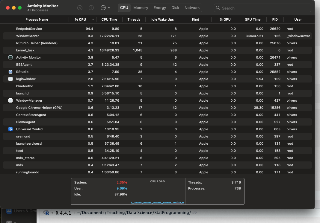
It shows the processes running at the time in the first column and the number of threads associated with the processes in the fourth column. For example, the (idle) R Studio process is consuming only 3.7% of available CPU and is running 35 threads. The kernel_task manages an impressive 1,045 threads.
In order to understand parallel programming, the simultaneous execution of multiple programming instructions, we need to cover some terminology first.
A process is a running program that has its own memory space. A process can be an entire application such as R Studio, a part of an application, or a service in the operating system. Processes are isolated from each other, if they need to share data, a form of inter-process communication such as a network socket must be established.
A thread is spawned by the process to perform a task and shares the memory space of the process. Threads that belong to the same process can directly communicate with each other and share data. Threads are used to execute a program asynchronously. For example, calculations can happen in one thread while another thread waits for user input.
A processor is the hardware that provides the infrastructure for processes to run. A process is software, a processor is hardware. Modern computers can have multiple processors, each processor with multiple cores. A system with 16 cores could be made from a single processor with 16 cores or 4 sockets with 4 cores, and so on. Larger servers have multiple sockets and can have hundreds of cores. For example, tinkercliffs1, a server in the Advanced Research Computing (ARC) facility at Virginia Tech has 2 sockets with 128 cores each, for a total of 256 cores. In addition to central processing units (CPUs), systems can have other processing units such as graphical processing units (GPUs) or tensor processing units (TPUs). For example, the Apple M2 Pro chip on this MacBook houses the following processors:
A cluster is a group of network-connected machines, either locally or remote. The machines in the cluster communicate via a network protocol and do not share memory resources. Compute clusters are common in high-performance computing (HPC) and in cloud computing. In HPC we often need to combine the massive compute powers across many large servers in order to solve difficult numerical problems. In cloud computing the large network of computers is used to solve many different but smaller problems simultaneously.
A node is a single machine in a cluster.
A forking operation clones a process along with its instructions and data. All forked processes see the same data if they read the data only. A copy of the data is made when the data are changed in some way. Forking is unique to POSIX operating systems (MacOS, Linux, Unix). An alternative to forking processes is starting a second, standalone process of the same kind. In this case, the two processes do not share the same data and instructions. On Windows system, creating separate processes that communicate over some protocol is the only way in which processes can be duplicated.
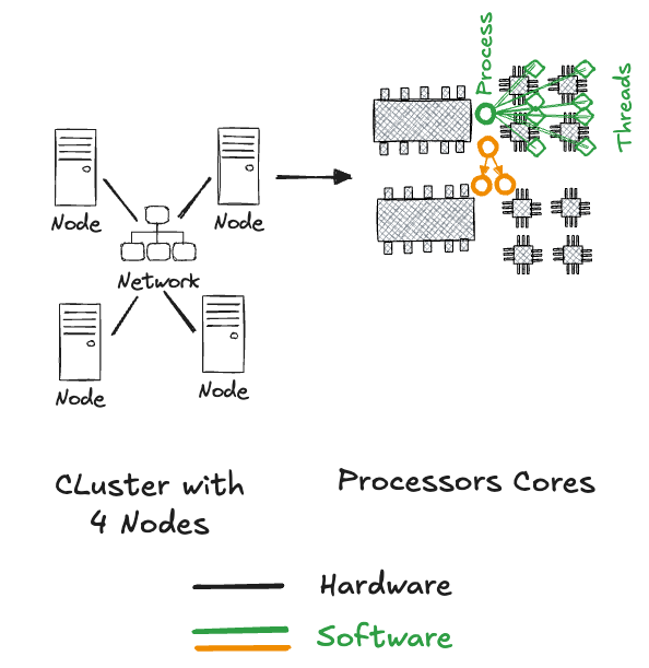
In summary, we can organize a high-performance computing environment as follows (Figure 11.2): a cluster of machines are connected via network; a node of the cluster has one or more processors, each with one or more cores. Processes are started on the processors to run programs, each process can spawn multiple threads and on some operating systems processes can be cloned by a process called forking.
Processes have multiple threads because they do lots of different things at the same time, such as performing calculations while processing user input or allowing you to scroll through an email while the Inbox updates. Without such asynchronous execution of tasks the user experience would be miserable. Tasks would be serialized and we would have to wait for one task to be completed before another can start. Or, we would have to stop a task after some processing, switch context to another task, complete a bit of that one, and switch back to the first.
In statistical computing we are also interested in parallel, asynchronous execution, with the important difference that the tasks are often identical.
Suppose you want to accumulate the \(\textbf{X}^\prime\textbf{X}\) matrix in a model where \(\textbf{X}\) is of size \((n \times p)\). In a serial execution model one thread would read each row of the data and accumulate the \(i=1,\cdots,n\) products \(\textbf{x}_i\textbf{x}_i^\prime\) and accumulate them: \[ \textbf{X}^\prime\textbf{X} = \sum_{i=1}^n \textbf{x}_i\textbf{x}_i^\prime \]
(Here, \(\textbf{x}_i\) is a \((p \times 1)\) column vector and \(\textbf{x}^\prime_i\) is a \((1 \times p)\) row vector.) In a parallel execution model using multiple threads we can partition the data into \(k\) subsets of sizes \(n_1, \cdots, n_k\) such that \(\sum_{j=1}^k n_j = n\). We would probably make the \(n_j\) as similar to each other as possible to give each thread the same amount of work. \(k\) threads would then accumulate a partial cross-product matrix based on the \(n_j\) observations that the \(j\)th thread sees: \[ \textbf{X}^\prime\textbf{X}^{(j)} = \sum_{i=1}^{n_j} \textbf{x}_{i}^{(j)} \textbf{x}_i ^{(j)\prime} \] The notation \(\textbf{x}_{i}^{(j)}\) depicts the \(i\)th observation in the batch for the \(j\)th thread and \(\textbf{X}^\prime\textbf{X}^{(j)}\) is the partial cross-product matrix formed by the \(j\)th thread.
At the end of the multithreaded execution we have \(k\) partial cross-product matrices and their sum yields the desired result: \[ \textbf{X}^\prime\textbf{X} = \sum_{j=1}^k \textbf{X}^\prime\textbf{X}^{(j)} \]
Which execution model is preferred? Single-threaded (serial) accumulation of a single cross-product matrix or multithreaded accumulation of \(k\) partial cross-product matrices that are then added up?
As always, the answer is “it depends”. Normally one would expect the threaded execution to perform faster than serially running through all observations, but multithreading is not without overhead. Creating threads requires computing resources. Each thread is provided with memory. If the number of columns \(p\) is large, then single-threaded execution allocates one cross-product matrix versus \(k\) matrices for threaded execution. One could allow the \(k\) threads to all write to the same memory, but that would require to lock threads, otherwise two threads might write simultaneously to the same memory location, trashing each other’s contributions. Such locking would limit the potential speedup from parallel execution. When the number of observations is small, the benefits of forming the partial cross-product matrices in parallel might be outweighed by the time and resources required to create, manage, and destroy the threads themselves.
If one uses a parallel execution model with forks rather than threads, or a socket-based execution model on a single machine, or a clustered execution model with multiple machines, the overhead is even greater than for the multithreaded model.
In short, parallel execution is typically advantageous and improves the performance of programs. However, it is not without overhead. And there are other issues to consider. For example, parallel execution does not guarantee that the operations occur in the same order. While mathematically equivalent, the sums
\[ \textbf{X}^\prime\textbf{X} = \sum_{i=1}^n \textbf{x}_i\textbf{x}_i^\prime \]
and
\[ \textbf{X}^\prime\textbf{X} = \sum_{j=1}^k \textbf{X}^\prime\textbf{X}^{(j)} \]
can differ computationally and the latter sum can change slightly from one run to the next.
And then, there is Amdahl’s law.
Named after the computer scientist Gene Amdahl, the law states that
the overall performance improvement gained by optimizing a single part of a system is limited by the fraction of time that the improved part is actually used
Suppose you are parallelizing a task that consist of two sub-tasks. Task A is inherently serial and cannot be parallelized. Task B can be parallelized. The overall speedup gained by parallelization depends on the fraction of the time spent with task A. If the non-parallelizable part of a program takes 80% of the runtime and you speed up the parallelizable part by 10x, the new program exeutes in 82% of the time of the original program. You did not gain much.
Amdah’s law is quite obvious. If there is a fixed cost for the non-modifiable part of a project you cannot get it any cheaper. The fixed cost sets a lower bound. Yet, in computer programming we often forget Amdahl’s law when efforts to optimize code (by parallelization or otherwise) focus on parts of the code that are really not a bottleneck. In the \(\textbf{X}^\prime\textbf{X}\) example, suppose that processing the vector multiplication \(\textbf{x}_i\textbf{x}_i^\prime\) is many times faster than retrieving a row of data from the storage device. The thread(s) computing the overall or the partial cross-product matrices would starve for data and sit idle until the next row arrives. The speed of data retrieval determines the performance of the algorithm.
RR is an interpreted language and as an R programmer you do not directly create, manage, and terminate threads within the R process. Parallelization through multithreading is done by the underlying code written in C or C++.
As R programmer, you mostly concentrate efforts to parallelize on what are called “embarrassingly parallel” problems, units of computations that you control that can be executed completely independently. A great example is the bootstrap. \(B\) samples are drawn with replacement from a data frame of size \(n\), a statistical method is applied to each bootstrap sample, and the \(B\) results are somehow aggregated. This process is “embarrassingly parallel” because you can draw and process the \(i\)th bootstrap sample independently of the \(j\)th sample. If overhead is low and processes can run at full blast, embarrassingly parallel problems can exhibit close to linear speedup compared to serial execution.
Because you cannot directly manage threads from the R session, parallel programming in R relies on forking or separate processes. On operating systems that support forking of processes (MacOS, Linux, Unix), copies of the current process are spawned via a system fork call. You can think of the forked processes as somewhat akin to the threads a low-level systems programmer would create in C or C++. However, the forked processes are separate processes while threads run within a given process. The fork has in common with threads that data and instructions are shared between the forked processes. Libraries you loaded prior to forking will also be available in the forked processes.
The basic packages in R for parallel program execution are parallel, foreach, and doParallel. The parallel package is part of basic R and combines functionality found earlier in the snow and multicore packages. multicore relies on forking processes, snow starts completely separate processes and and uses sockets, parallel virtual machines (PVM), message passing interface (MPI), or NetworkSpaces (NWS) for parallelization. By combining snow and multicore, the parallel library supports parallel execution on POSIX and non-POSIX (Windows) operating systems. The flip side of this flexibility is that you need to let the library know which parallelization protocol to follow.
Packages like caret take advantage of parallel execution if the appropriate backend parallelization mechanism is in effect—more on that below.
multidplyr is a backend for dplyr that partitions a data frame across multiple cores.
foreach and doParallel PackagesA great way of getting started with parallelizing R code is the foreach package in combination with the doParallel package.
foreachforeach provides a new looping construct that supports parallel execution of the loop body. You combine a call to foreach with the binary %do% operator to run the loop. Unlike the for loop, foreach acts like a function that returns a result.
Consider the following example:
library(foreach)
b <- seq(10,12)
foreach(a=1:3) %do% (a+b)[[1]]
[1] 11 12 13
[[2]]
[1] 12 13 14
[[3]]
[1] 13 14 15foreach iterates over the variable a and adds its value to the vector b = [10, 11, 12]. The result is returned in the form of a list, which is efficient but might not be the most convenient form to work with. Using the .combine option of foreach, you can control the format of the result.
foreach(a=1:3, combine='c') %do% (a+b)[[1]]
[1] 11 12 13.combine='c' instructs foreach to use the standard c() function in R to concatenate the results. You could also use .combine='cbind' or .combine='rbind', even operators such as + or * to combine results.
Notice in the results above that b is not being iterated over, it is a global variable outside of the loop. Each iterate, a=1, a=2, a=3 is applied to the entire vector b. If you place b inside the foreach operator, then it is also iterated over, returning a scalar result for each iterate
foreach(a=1:3, b=seq(10,12), .combine='c') %do% (a+b)[1] 11 13 15Here is an example of using the + operator to add up random numbers generated in a loop:
set.seed(654)
foreach(i=1:10, .combine="+") %do% rnorm(5)
[1] -1.1806931 -3.1580865 1.9819221 1.1011581 -0.3506018doParallelSo far, the foreach loops executed sequentially. To move to parallel execution, replace the %do% operator with the %dopar% operator. However, we have to do a little more setup work, we have to tell R what parallelization backend to use. This is where the doParallel package comes in.
This R session runs on a multicore processor and I want to use multicore functionality rather than creating a cluster. The first question is, how many cores are available for parallel execution.
library(parallel)
detectCores()
[1] 12Nice, that is a lot of cores, let’s use 4 of them.
The following statements load the doParallel library and register a parallel backend with the registerDoParallel function. The first argument to registerDoParallel is a cluster object, the second argument is the number of cores to use. In this example, the first argument is omitted. On a POSIX machine (like this MacBook) this results in multicore execution on a single node, forking four processes. On a Windows machine this results in a three-node cluster unless you provide the number of machines in makeCluster (see below).
library(doParallel)
registerDoParallel(cores=4)
getDoParWorkers()
[1] 4getDoParName()[1] "doParallelMC"getDoParName() confirms that we are using the multicore parallel backend.
If you want to set up a cluster for parallelization instead, the steps are
makeCluster, choosing type="PSOCK" for socket-based clusters or type="FORK" for forked clusters.registerDoParallelstopCluster()cl <- makeCluster(2, type="PSOCK")
registerDoParallel(cl)
## Do your parallel work
stopCluster(cl)The previous code chunk is for illustration and was not executed, so we still have a multicore parallel backend in effect. We can now finally run code in parallel by switching from %do% to the %dopar% operator:
set.seed(654)
system.time(
    x <- foreach(i=1:10000, .combine="+") %dopar% rnorm(5)
)
user system elapsed
0.661 0.052 0.658 x[1] -80.08174 -24.44327 18.76143 56.78028 113.11059Let’s run this again:
set.seed(654)
system.time(
    x <- foreach(i=1:10000, .combine="+") %dopar% rnorm(5)
)
user system elapsed
0.646 0.071 0.633 x[1] -45.810674 -66.404293 5.376642 -241.933774 13.602749Whoa!
We are already seeing one issue with parallel execution. Despite having set a seed for the random number generator, each call to foreach generates a different result. Somehow the random number streams are not the same in the forks of the process. You can see this by comparing the output from the following two code chunks:
set.seed(654)
foreach(i=1:6, .combine="rbind") %dopar% rnorm(5)
[,1] [,2] [,3] [,4] [,5]
result.1 -0.2150568 -1.6594724 -0.3972224 -1.3073994 0.88945393
result.2 -0.9349796 1.6054302 0.7673148 1.2438284 -0.66669577
result.3 -1.4521076 -0.0955965 -2.1741048 0.6564282 -0.06955734
result.4 0.6225284 0.6658790 -1.4487674 -0.1131063 -1.16335908
result.5 -0.7327858 -0.2371235 1.7549391 -0.9418489 0.60785157
result.6 1.1961404 -1.4246921 0.8058946 1.2281679 0.15233176set.seed(654)
foreach(i=1:6, .combine="rbind") %dopar% rnorm(5) [,1] [,2] [,3] [,4] [,5]
result.1 -2.2379920 0.2866470 -0.3471283 -0.4175620 0.8067311
result.2 -1.0876835 0.2516772 -0.0670123 0.2083480 -0.5253229
result.3 1.1509832 -0.1054614 1.4840200 -1.0383844 -0.3778725
result.4 1.0667234 0.5417052 -1.1420096 -0.9119156 -0.7855920
result.5 -2.5232488 -1.1561825 -0.4338535 -0.6516571 0.8006728
result.6 -0.4405905 -0.2377512 -3.6803450 2.1532061 -0.7691100If we use %do% and resort to serial execution instead, the random number streams are identical, as expected.
set.seed(654)
foreach(i=1:6, .combine="rbind") %do% rnorm(5)
[,1] [,2] [,3] [,4] [,5]
result.1 -0.76031762 -0.38970450 1.689625228 -0.0942356 0.09530146
result.2 0.81727228 1.06576755 0.939845633 0.7412122 -0.43531214
result.3 -0.10726012 -0.83816833 -0.982605890 -0.8203710 -0.87143256
result.4 -0.06097056 0.01388045 -0.006557849 0.6616963 -0.76282807
result.5 -0.28669247 0.12135500 0.512579937 0.7221273 -0.43699928
result.6 -0.83605962 -0.62698452 0.774016151 -0.6918666 1.02610364set.seed(654)
foreach(i=1:6, .combine="rbind") %do% rnorm(5) [,1] [,2] [,3] [,4] [,5]
result.1 -0.76031762 -0.38970450 1.689625228 -0.0942356 0.09530146
result.2 0.81727228 1.06576755 0.939845633 0.7412122 -0.43531214
result.3 -0.10726012 -0.83816833 -0.982605890 -0.8203710 -0.87143256
result.4 -0.06097056 0.01388045 -0.006557849 0.6616963 -0.76282807
result.5 -0.28669247 0.12135500 0.512579937 0.7221273 -0.43699928
result.6 -0.83605962 -0.62698452 0.774016151 -0.6918666 1.02610364Fortunately, the iterators library provides functions that create special iterators, such as iterating while generating random numbers. Using the inorm() iterator, the random number streams are reproducible under parallel execution:
library(iterators)
set.seed(543)
foreach(a=irnorm(4, count=6), .combine='rbind') %dopar% a
[,1] [,2] [,3] [,4]
result.1 1.3514112 0.1854795 0.43152654 -0.190607458
result.2 -0.9715509 0.7680671 -0.17847276 -0.004322258
result.3 1.6597295 -0.6560060 -0.48553128 -0.776180044
result.4 -0.1912907 0.3017708 0.05322434 0.094927358
result.5 -0.2223354 0.1900994 0.30463665 -0.981463360
result.6 -1.3398361 -1.4437327 0.35197447 0.116163784set.seed(543)
foreach(a=irnorm(4, count=6), .combine='rbind') %dopar% a [,1] [,2] [,3] [,4]
result.1 1.3514112 0.1854795 0.43152654 -0.190607458
result.2 -0.9715509 0.7680671 -0.17847276 -0.004322258
result.3 1.6597295 -0.6560060 -0.48553128 -0.776180044
result.4 -0.1912907 0.3017708 0.05322434 0.094927358
result.5 -0.2223354 0.1900994 0.30463665 -0.981463360
result.6 -1.3398361 -1.4437327 0.35197447 0.116163784Finally, let’s return to our first %dopar% example and compare the performance to serial execution with %do%:
set.seed(654)
system.time(
    x <- foreach(i=1:10000, .combine="+") %do% rnorm(5)
)
user system elapsed
0.706 0.001 0.707 x[1] 177.89020 -138.02384 106.18030 121.00753 -62.05028Well, darn. All this work and there was not much of a speedup. The elapsed time is the wall-clock time that expired during the run, this is what you want to look at here. Maybe we need to give the parallel processes more work to experience the speedup from parallel execution—a more substantial analysis is called for.
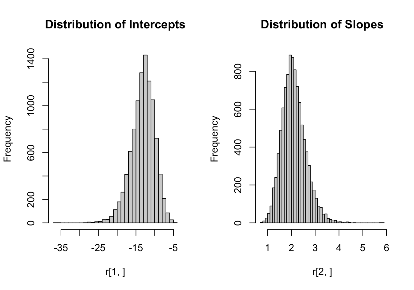
Here is a more substantial example of parallel execution. We are interested in the distribution of the intercept and slope of a logistic regression where the target variable is the iris species in the iris data set and the predictor variable is sepal length. Observations for Iris setosa are removed from the data set to reduce the number of levels in Species to two.
The following code computes 10,000 bootstrap estimates using foreach and multicore parallelization. You should try this on your machine, but on this MacBook the bootstrap loop executes 3 times faster (with 4 worker processes) compared to serial execution. That is not bad! A 4x speedup would mean linear scaling and typically cannot be expected from forked processes, even for embarrassingly parallel problems.
data(iris)
df <- iris[which(iris[,5] != "setosa"), c(1,5)]
n <- dim(df)[1]
B <- 10000

print(system.time(
r <- foreach(icount(B), .combine='cbind') %dopar%
    {
        bstrap <- sample(n, n, replace=TRUE)
        coefficients(glm(Species ~ Sepal.Length,
                         data=df[bstrap,],
                         family=binomial(logit)))
    }
))
user system elapsed
6.456 0.289 1.982 Figure 11.3 displays the bootstrap distributions of the logistic parameter estimates.
A random forest is essentially a bootstrap of decision trees where the trees are constructed by introducing another random element. At each split of a tree not all possible predictors are evaluated, but a random sample of them. The best predictor among the randomly chosen ones is then used to split the tree at this level. The additional variability introduced by randomizing the splits makes random forests more effective than bagged trees, which are just bootstrapped trees. Whether bagging trees or building a random forest, the process involves constructing many individual trees, which are then combined to make a prediction or classification.
The individual trees are constructed independently of each other, which allows for parallelization. To demonstrate, we are following an example in the foreach vignette. First, we simulate a data set with 100 rows and 5 columns and a categorical target vector with two levels.
set.seed(54)
x <- matrix(runif(500), 100)
y <- gl(2, 50)
To build a random forest of 1,000 trees, we can call randomForest in the randomForest package with the ntree=1000 option, or we can build 4 forests of 250 trees each, and combine them. This is where foreach comes in.
Before we can build four forests of 250 trees each in parallel, there are two issues to deal with:
We need to figure out how to combine the results from the four calls to randomForest. The return object from that function is rather complicated. Fortunately, the randomForest library provides a combine function to combine two or more ensembles of trees into a single one.
The randomForest library was not loaded when the worker processes were forked at the time registerDoParallel was called. Loading the library now in the R session where foreach is called will not do the same in the forked processes. Use the .packages= option of foreach to request loading of needed packages in the worker processes
library(randomForest)
rf <- foreach(ntree=rep(250, 4),
              .combine=combine,
              .packages='randomForest') %dopar%
    randomForest(x, y, ntree=ntree)
#rfSuppose the program involves an inner and an outer loop. Something like this:
for (j in 1:length(a)) {
    for (i in 1:length(b)) {
        # do some work here
  }
}
If you convert this to parallel execution, which loop should you parallelize? Since we want to make sure to give our worker processes something substantial to chew on, the usual recommendation is to parallelize the outer loop. But if the outer loop has only a few iterations you might not get to use all cores.
Further, if the inner and outer loops can be executed independently, that is, the code is embarrassingly parallel across both loops, then it would be nice if we can parallelize across both loops simultaneously. This is where the nested loop operator %:% in foreach comes in. %:% works in conjunction with %do% or %dopar%, so it does not require parallel execution. You can use the operator to draw on foreach functionality to write elegant and efficient code:
foreach(j=b, .combine='cbind') %:%
    foreach(i=a, .combine='c') %do% {
      # do some work here
    }
See this vignette for more details on the nested for loop operator %:%.
The following example is modified from cross.R here.
The data consists of 500 observations on one continuous target variable y and 100 possible predictor variables x.1 – x.100. We wish to examine a series of 100 regression models: \[
y = \beta_0 + \beta_1 x_1 + \epsilon
\] all the way to
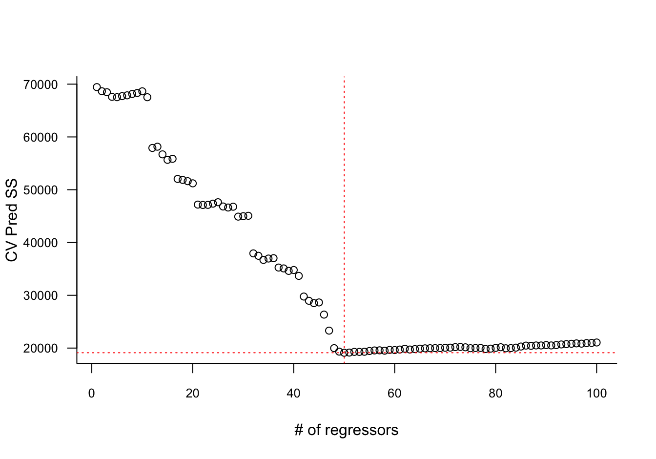
\[ y = \beta_0 + \beta_1 x_1 + \cdots + \beta_{100}x_{100} + \epsilon \] For each of those regression models we compute the prediction error sum of squares by 10-fold cross-validation. That means we partition the data into 10 groups (called folds), fit the model 10 times, each time leaving out one of the folds and computing the prediction sum of squares for the observations left out. After the last fold has been processed, the 10 prediction sum of squares for the folds are summed or averaged to get the estimate for the entire data set.
This can be organized into two nested loops, one loop over the regression models and one loop over the folds. This results in 100 cross-validated prediction sum of squares values. The model that has the smallest value is the one that generalizes best to new observations (Figure 11.4).
n_rows <- 500
n_cols <- 100
n_folds <- 10

set.seed(5432)
xv <- matrix(rnorm(n_rows * n_cols), n_rows, n_cols)
beta <- c(rnorm(n_cols / 2, 0, 5),
          rnorm(n_cols / 2, 0, 0.25))
yv <- xv %*% beta + rnorm(n_rows, 0, 20)
dat <- data.frame(y=yv, x=xv)
folds <- sample(rep(1:n_folds, length=n_rows))

# .final= specifies a function to process the final result

print(system.time(
prss <-
    foreach(i=2:(n_cols+1), .combine='c') %:%
        foreach(fold=1:n_folds, .combine='c', .final=mean) %dopar% {
           glmfit <- glm(y ~ ., data=dat[folds != fold, 1:i])
           yhat <- predict(glmfit, newdata=dat[folds == fold, 1:i])
           sum((yhat - dat[folds == fold, 1]) ^ 2)
    }
))
user system elapsed
6.389 0.220 1.736 plot(prss,
las=1,
xlab="# of regressors",
ylab="CV Pred SS",
bty="l",
cex.axis=0.8)
abline(h=min(prss), col="red",lty="dotted")
abline(v=which.min(prss),col="red",lty="dotted")