Like other unsupervised learning methods, Association Rule Mining (ARM) tries to learn aspects of the joint density \(p(\textbf{X})\) of the data. It specifically asks if in regions of \(p(\textbf{X})\) where the density is high, are certain values of \(X_j\) associated with values of \(X_j\) more frequently than one would expect under a completely random allocation? In other words, are there associations between the values that tell us something interesting about the joint distribution of the data?
The most frequent form of ARM is market basket analysis, the name appeals to items a customer places in a shopping basket. \(X_1, \cdots, X_p\) are the possible items offered for purchase, \(X_j \in \{0,1\}\). \(X_{ij}\) takes on the value \(1\) if the \(i\)th customer selects the \(j\)th item into their basket, \(0\) otherwise. Market basket analysis is concerned with the properties of the \((n \times p)\) matrix \(\textbf{X}\) of zeros and ones, trying to understand with items are purchased together—the famous example is beer and diapers.
Customer segmentation: grouping customers based on their buying behavior
Retail allocation: which item should be on shelves and how should they be grouped
Recommender systems: cross-marketing of products
Survey analysis: which responses go together?
Precursor analytics: Borne (2021) mentions this interesting application of ARM, where data are time stamped. The analysis seeks time lags at which the association strength peaks. Precursor analysis has found that solar storm events show the strongest geomagnetic effects 2–3 hours after the storm and that video cameras are bought 3 months after the purchase of a video (VHS) player.
The approach to association rule mining is essentially mode hunting, looking for areas of the joint distribution with high densities and finding associations of items that are more frequent than expected if shopping baskets were filled at random. This is conceptually pretty simple, it is just a matter of counting.
Example: Beers and Diapers
Borne (2021) cites beer–diaper association as the classic example of market basket analysis, although the particular example might be more legend than reality.
Suppose that a retail store has 600,000 transactions (shopping baskets). 7,500 (1.25%) of the shopping baskets contain diapers, 60,000 (10%) of the baskets contain beer. So we know that a basket is 8 times more likely to contain beer than diapers. In order to analyze the association of beer and diapers we need to know how many of the baskets contain both. Suppose that number is 6000 (1%).
If beer and diaper purchases were independent, then 10% of the diaper purchases would be accompanied by beer purchases, or, equivalently, 1.25% of beer buyers would pick up diapers. Either way, under independence of the two items we would expect \(600,000 \times 0.1 \times 0.0125 = 750\) baskets with both beer and diapers. The actual number of baskets containing both is much higher.
The ratio between what was observed and what was expected under independence is called the lift factor: \[
L = \frac{6000}{750} = 8
\]
Association rule mining is about finding associations that have a large lift factor. But that is not the only criterion by which associations are judged. A lift factor of 10 is very interesting when the items appear frequently in baskets, but not that interesting if they are purchased very rarely. In the former case one can focus promotional pricing on those items together whereas in the latter case this might not yield a lot of bang for the buck (literally).
Finding meaningful associations can be challenging, since we are dealing with a \(p\)-dimensional distribution and \(p\) can be very large. Market basket analysis of Amazon.com involves more than 12 million products. The data are very sparse, many items are never purchased together. There is insufficient data to estimate proportions reliably. Also, we would not be interested only in associations between two items; what about sets of three or four or more items? We need a structured approach and simplify the procedure—this leads us down the path of item sets.
27.2 Association Rules and Item Sets
Items are collected in item sets, for example {butter, bread} is a two-item set and {milk} is a single-item set. Association rules display relationships among item sets, for example
{bread, butter} \(\Rightarrow\) {jelly}
The left hand side (lhs) of the rule is called the head or the antecedent, the right hand side (rhs) is called the body or the consequent of the rule. The rule is read as follows: if the head (lhs) occurs then the body (rhs) also occurs.
The most important metrics by which to judge an association rule are its support, confidence, and lift.
Support
Suppose we have \(n\) transactions and a rule $A \(\Rightarrow\) B$ where A and B are item sets. Let \(\#A\) denote the number of times A occurs in the database and \(\#(A,B)\) the number of times the the sets A and B occur together. For example, if A is a three-item set, then \(\#A\) is the number of records where all three items are present. if B is a single-item set, then \(\#(A,B)\) is the number of records where all four items are present.
The support of the rule is the relative frequency with which head and body appear: \[
S(A \Rightarrow B) = \frac{\#(A,B)}{n}
\]
Confidence
The confidence of the rule is the estimate of the conditional probability to find the body (the consequent) of the rule in transactions given that they contain the head (the antecedent):
\[
C(A \Rightarrow B) = \frac{\#(A,B)}{\#A}
\] It is a measure of predictability of the association between A and B.
Support can be beneficial for finding the connection between products in comparison to the whole database, whereas confidence looks at the connection between item sets. A support threshold is often used to focus on those item sets that are interesting because they are frequent. For example, a support threshold of 0.2 implies that only item set that appear in at least 20% of the transactions are considered. The confidence, on the other hand, tells us how likely it is that B occurs every time A occurs.
It is possible that confidence is high but support is low. For example, {caviar} \(\Rightarrow\) {vodka} is a high-confidence rule, because given that caviar is purchased it is likely to be accompanied by a vodka purchase. It is a low-support rule because caviar is not purchased frequently. An algorithm that sets a support threshold might miss association rules with low-support and high confidence.
A rule can have 100% confidence if the head requires the body—that is, every time the head occurs the body also occurs. For example, if opening a savings account requires having a checking account, then \[
C(\text{savings} \Rightarrow \text{checking}) = \frac{\#(\text{checking and savings})}{\#\text{savings}}=1
\] Knowing that a customer has a savings account, you can say with certainty that they also have a checking account. The body (checking account) is completely predictable from the head (savings account).
Lift
The lift of an association rule measured how much more likely the association is compared to independence of the items: \[
L(A \Rightarrow B) = n \frac{\#(A,B)}{\#A \#B} = \frac{C(A\Rightarrow B)}{S(B)}
\] The lift factor is an estimate of the ratio of the joint probabilities \[
\frac{\Pr(A,B)}{\Pr(A)\Pr(B)}
\]
When \(L(A \Rightarrow B) = 1\), A and B are not associated with each other (independent).
When \(L(A\Rightarrow B) > 1\), then A and B occur more frequently together than under a random selection of items—A and B have a positive association.
When \(L(A \Rightarrow B) < 1\), then A and B occur less frequently together than expected under a random selection of items—A and B have a negative association.
Example
A supermarket has 80 shopping baskets, 60 of them contain bread, 50 contain peanut butter. 40 baskets contain both bread and peanut butter.
Lift for rule {bread} \(\Rightarrow\) {peanut butter} = 80 x 40 / (60 x 50) = 1.06
Another example calculation follows before we apply an efficient algorithm to find rules in a large database.
Example
Suppose we have indicator variables \(X_1, \cdots, X_5\) for five items and the following baskets
Basket
\(X_1\)
\(X_2\)
\(X_3\)
\(X_4\)
\(X_5\)
1
1
1
1
0
0
2
1
0
1
1
0
3
0
1
1
1
0
4
1
0
0
1
1
5
0
1
1
0
1
The next table shows support, confidence, and lift for a series of rules
Rule
Support
Confidence
Lift
\(X_1 \Rightarrow X_4\)
2/5
2/3
10/9
\(X_3 \Rightarrow X_1\)
2/5
2/4
5/6
\(X_1 \Rightarrow X_3\)
2/5
2/3
5/6
\((X_2,X_3) \Rightarrow X_4\)
1/5
1/3
5/9
27.3 Apriori Algorithm
The math to compute support, confidence, and lift of rules is simple, it just means counting occurrences in a database of transactions. What makes ARM tricky is the large number of rules. For \(p\) items, there are \(2^p-1\) non-empty item sets. An algorithmic approach is needed to find interesting rules, especially when \(p\) and \(n\) are large.
Also, we want to query the database with queries such as
Find all rules that have “bagels” in the antecedent. Find all rules that have “sausage” in the antecedent and “mustard” in the consequent.
Caution
When analyzing large databases of baskets, you will find a large number of spurious associations. Those occur when items appear together more frequently compared to independence, but only by chance. Suppose we apply a 5% significance rule, meaning that we declare associations as “significant” if they appear beyond the 95th percentile of the frequency distribution. A market basket analysis with 1,000,000 two-item sets in which there are no associations whatsoever will declare 50,000 associations as “significant” although none of them are relevant.
The Apriori algorithm of Agrawal, Imieliński, and Swami (1993) is based on setting a support threshold \(s\) and a confidence threshold \(c\). Multiple passes over the data are made. In the first pass the support of single-item sets is computed and any items with \(S(A) < s\) are discarded. In the second pass the support of two-item sets is computed and any sets with \(S(A,B) < s\) are again discarded. This continues until all candidate rules in a pass have support less than \(s\).
Based on the item sets determined so far, only those association rules are displayed for which the confidence exceeds the threshold \(c\).
The Apriori algorithm makes it feasible to find relevant association rules in very large databases. It works because \(S(A,B) \le \min(S(A),S(B))\), in other words the support of any sets found on a subsequent pass cannot exceed the support of the subsets of the previous pass. However, the algorithm also has some disadvantages:
It can create large candidate sets of rules and thus lead to many spurious rules.
It requires a query engine to filter and summarize candidate item sets.
It passes through the database multiple times, once for each cardinality of item sets.
It is unlikely to find rules with high confidence and low support because items are filtered first based on the support threshold—only item sets that pass this threshold are considered in computing confidence, which is a measure comparing item sets.
Example Analysis with arules
Example: Grocery Shopping
The apriori function in the arules package in R performs association rule mining based on the Apriori algorithm. The input data to the function is an object of class transactions, which is based on a sparse matrix representation of item occurrences.
We analyze here the Groceries data set that is part of the arules package. This data set contains 1 month (30 days) of real-world point-of-sale transaction data from a typical local grocery outlet. The data set contains 9835 transactions and the items are aggregated into 169 categories.
library(arules)data(Groceries)summary(Groceries)
transactions as itemMatrix in sparse format with
9835 rows (elements/itemsets/transactions) and
169 columns (items) and a density of 0.02609146
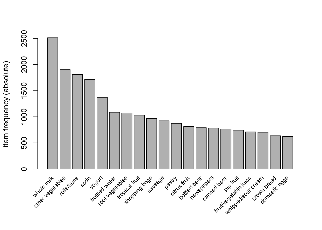
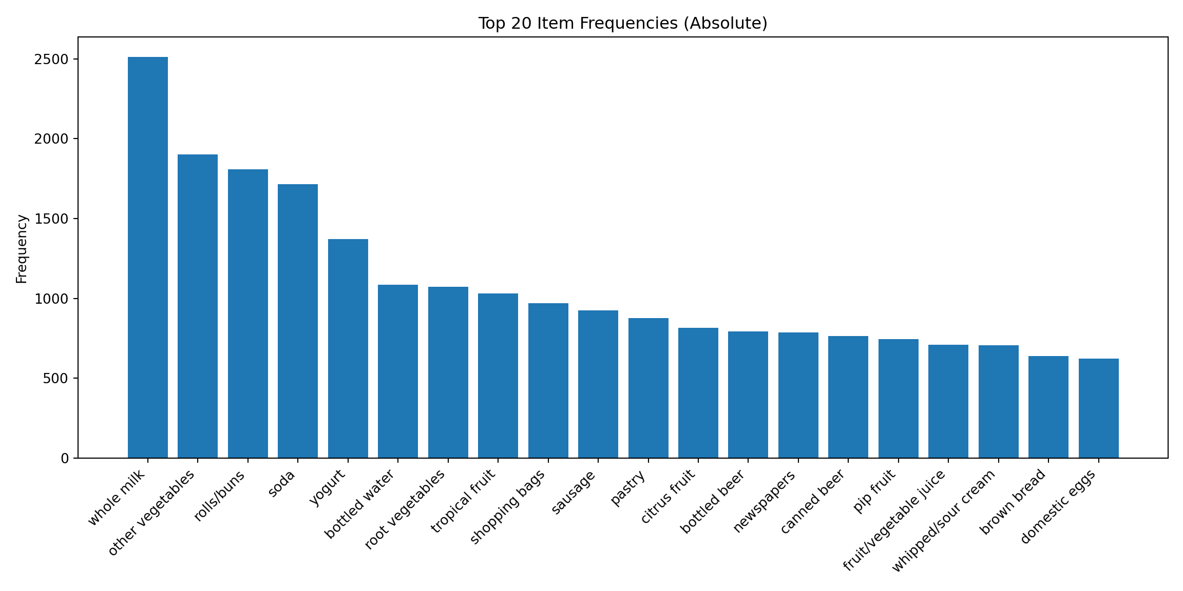
most frequent items:
whole milk other vegetables rolls/buns soda
2513 1903 1809 1715
yogurt (Other)
1372 34055
element (itemset/transaction) length distribution:
sizes
1 2 3 4 5 6 7 8 9 10 11 12 13 14 15 16
2159 1643 1299 1005 855 645 545 438 350 246 182 117 78 77 55 46
17 18 19 20 21 22 23 24 26 27 28 29 32
29 14 14 9 11 4 6 1 1 1 1 3 1
Min. 1st Qu. Median Mean 3rd Qu. Max.
1.000 2.000 3.000 4.409 6.000 32.000
includes extended item information - examples:
labels level2 level1
1 frankfurter sausage meat and sausage
2 sausage sausage meat and sausage
3 liver loaf sausage meat and sausage
The data are very sparse, which is typical for these applications. Only 2.6% of the 9835 x 169 possible item–transaction combinations are non-zero. The most frequently item is whole milk, its support is 2513/9835 = 0.255516. There are 2159 single-item sets, 1643 two-item sets, and one 32-item set. The median item set size is 3.
You can query the raw data for the transactions with the inspect function:
The first transaction involves four items, the second transaction two items, the third transaction was a purchase of whole milk alone.
The itemFrequencyPlot function helps to inspect the frequency distribution of the items in the database. The following call requests the 20 items with the highest absolute frequency.
By default, the apriori function mines for rules with a support of \(s > 0.1\) and a confidence of \(c > 0.8\). The following call changes these values. Based on the summary above, it should only find three rules in the database, based on single-item sets for whole milk, other vegetables, and rolls/buns.
As expected, only three rules are found by the algorithm since only three single items exceed the support threshold of 0.18. It would have been possible to find rules based on two-item sets constructed from whole milk, other vegetables or rolls\buns on the second pass, but none of those combinations had support > 0.18.
The head of the rules is displayed as lhs and the body as rhs for the left hand side and right hand side of the rule, respectively. The coverage is the support of the lhs which shows that the set {} is to be interpreted as all transactions. That also explains why the confidence of the single-item rules is equal to their support.
Changing the value for support to a smaller number generates more rules.
set of 410 rules
rule length distribution (lhs + rhs):sizes
3 4 5 6
29 229 140 12
Min. 1st Qu. Median Mean 3rd Qu. Max.
3.000 4.000 4.000 4.329 5.000 6.000
summary of quality measures:
support confidence coverage lift
Min. :0.001017 Min. :0.8000 Min. :0.001017 Min. : 3.131
1st Qu.:0.001017 1st Qu.:0.8333 1st Qu.:0.001220 1st Qu.: 3.312
Median :0.001220 Median :0.8462 Median :0.001322 Median : 3.588
Mean :0.001247 Mean :0.8663 Mean :0.001449 Mean : 3.951
3rd Qu.:0.001322 3rd Qu.:0.9091 3rd Qu.:0.001627 3rd Qu.: 4.341
Max. :0.003152 Max. :1.0000 Max. :0.003559 Max. :11.235
count
Min. :10.00
1st Qu.:10.00
Median :12.00
Mean :12.27
3rd Qu.:13.00
Max. :31.00
mining info:
data ntransactions support confidence
Groceries 9835 0.001 0.8
call
apriori(data = Groceries, parameter = list(support = 0.001, conf = 0.8), control = list(verbose = F))
This query generated 410 rules, four-item rules most frequent among them. Their confidence ranges from 0.8 to 1.0, their lift ranges from 3.131 to 11.235.
The association with the highest lift factor is the purchase of beer when the basket contains liquor and wine. The confidence of this transaction is very high, making beer purchase highly predictable from the presence of liquor and wine.
You can limit the maximum length of rules generated with the maxlen= parameter. Setting the maximum length to 3 reduces the number of generated ruls to 29.
# setting max length of rules to 3rules <-apriori(Groceries, parameter =list(supp=0.001, conf=0.8,maxlen=3),control =list(verbose=F))summary(rules)
set of 29 rules
rule length distribution (lhs + rhs):sizes
3
29
Min. 1st Qu. Median Mean 3rd Qu. Max.
3 3 3 3 3 3
summary of quality measures:
support confidence coverage lift
Min. :0.00102 Min. :0.800 Min. :0.00112 Min. : 3.13
1st Qu.:0.00112 1st Qu.:0.812 1st Qu.:0.00122 1st Qu.: 3.26
Median :0.00122 Median :0.846 Median :0.00153 Median : 3.61
Mean :0.00147 Mean :0.861 Mean :0.00173 Mean : 4.00
3rd Qu.:0.00173 3rd Qu.:0.909 3rd Qu.:0.00214 3rd Qu.: 4.20
Max. :0.00254 Max. :1.000 Max. :0.00315 Max. :11.24
count
Min. :10.0
1st Qu.:11.0
Median :12.0
Mean :14.5
3rd Qu.:17.0
Max. :25.0
mining info:
data ntransactions support confidence
Groceries 9835 0.001 0.8
call
apriori(data = Groceries, parameter = list(supp = 0.001, conf = 0.8, maxlen = 3), control = list(verbose = F))
An application of the querying engine is to target items. For example, if folks are buying whole milk, what are they also buying? Report the 5 associations with the highest lift:
arulesViz::plot has specialized plotting methods for association rules. method="scatterplot" requires two quality measures and shades the rules by a third variable (lift is the default). method="matrix" arranges the rules by antecedent (head, lhs) and consequent (body, rhs).
Agrawal, Rakesh, Tomasz Imieliński, and Arun Swami. 1993. “Mining Association Rules Between Sets of Items in Large Databases.” In Proceedings of the 1993 ACM SIGMOD International Conference on Management of Data, 207–16. SIGMOD ’93. New York, NY, USA: Association for Computing Machinery. https://doi.org/10.1145/170035.170072.