Bagging is a general technique–like cross-validation–that can be applied to any learning method. It is particularly effective in ensembles of base learners with high variability and low bias. The name is short for bootstrap aggregating and describes its relationship to the bootstrap. Draw \(B\) bootstrap samples from the dataframe with \(n\) observations, fit a base learner to each of the \(B\) samples, and combine the individual predictions or classifications.
In the regression case, the \(B\) predictions are averaged, in the classification case the majority vote is taken to assign the predicted category.
Not surprisingly, bagging is popular with decision trees, unbiased regression or classification methods that tend to have high variability. A single decision tree might have a large classification or prediction error, an ensemble of 500 trees can be a very precise predictor. Random forests (Section 20.4) are a special version of bagged trees.
Bagging can be useful with other estimators.
Example: Bagging a Naive Estimator
Suppose we have 100 observations from a G(\(\mu\),2) distribution.
We want to estimate the mean of the normal, so the sample mean \[
\overline{Y} = \frac{1}{n} \sum_{i=1}^n Y_i
\] is the best estimator.
We can get close to that estimator by bagging a highly variable estimator, say the average of the first three observations. if \(Y_{(i)}\) denotes the \(i\)th observation in the data set, then \[
Y^* = \frac{1}{3} \sum_{i=1}^3 Y_{(i)}
\] is also an unbiased estimator for \(\mu\) and has standard deviation \[
\sqrt{\frac{\sigma^2}{3}} = 0.816
\] compared to the standard deviation of the sample mean, \[
\sqrt{\frac{\sigma^2}{100}} = 0.1414
\]
\(Y^*\) is more variable than \(\overline{Y}\) and both are unbiased estimators. The precision of estimating \(\mu\) based on \(Y^*\) can be improved by bagging the estimator: rather than compute \(Y^*\) once from the data, we compute it \(B\) times based on bootstrap samples from the data and take the average of the bootstrapped estimates as our estimate of \(\mu\).
set.seed(542)n <-100x <-rnorm(n, mean=0, sd=sqrt(2))bagger <-function(x,b=1000) { n <-length(x) sum_bs <-0 sum_bs2 <-0for (i in1:b) {# Draw a bootstrap sample bsample <-sample(n,n,replace=TRUE)# Compute the estimator est <-mean(x[bsample][1:3])# Accumulate sum and sum of squared value of estimator# so we can calculate mean and standard deviation later sum_bs <- sum_bs + est sum_bs2 <- sum_bs2 + est*est }# Compute mean and standard deviation of the estimator mn = sum_bs / b sdev =sqrt((sum_bs2 - sum_bs*sum_bs/b)/(b-1))return (list(B=b, mean=mn, sd=sdev))}cat("The best estimate of mu is ", mean(x),"\n\n")
The best estimate of mu is -0.004722246
l <-list()l[[length(l)+1]] <-bagger(x,b=10)l[[length(l)+1]] <-bagger(x,b=100)l[[length(l)+1]] <-bagger(x,b=1000)l[[length(l)+1]] <-bagger(x,b=10000)l[[length(l)+1]] <-bagger(x,b=25000)l[[length(l)+1]] <-bagger(x,b=50000)do.call(rbind.data.frame, l)
import numpy as npimport pandas as pd# Set random seednp.random.seed(542)# Generate datan =100x = np.random.normal(loc=0, scale=np.sqrt(2), size=n)def bagger(x, b=1000):""" Bootstrap aggregation function """ n =len(x) sum_bs =0 sum_bs2 =0for i inrange(b):# Draw a bootstrap sample bsample = np.random.choice(n, size=n, replace=True)# Compute the estimator (mean of first 3 elements) est = np.mean(x[bsample][:3])# Accumulate sum and sum of squared values sum_bs += est sum_bs2 += est * est# Compute mean and standard deviation of the estimator mn = sum_bs / b sdev = np.sqrt((sum_bs2 - sum_bs * sum_bs / b) / (b -1))return {'B': b, 'mean': mn, 'sd': sdev}print(f"The best estimate of mu is {np.mean(x):.6f}\n")
The best estimate of mu is 0.090683
# Run bagger with different b valuesl = []l.append(bagger(x, b=10))l.append(bagger(x, b=100))l.append(bagger(x, b=1000))l.append(bagger(x, b=10000))l.append(bagger(x, b=25000))l.append(bagger(x, b=50000))# Print resultsfor result in l:print(f"B={result['B']}, mean={result['mean']:.6f}, sd={result['sd']:.6f}")
The bagger function returns the mean and standard deviation of the \(B\) bootstrap estimates. Notice that by increasing \(B\), the bagged estimate gets closer to the optimal estimator, \(\overline{Y}\). The standard deviation of the bagged estimate stabilizes around 0.8, close to the theoretically expected value of \(\sqrt{2/3} = 0.816\). Both quantities returned from bagger are becoming more accurate estimates as \(B\) increases. The standard deviation of the bootstrap estimate does not go to zero as \(B\) increases, it stabilizes at the standard deviation of the estimator.
20.2 Why and When Does Bagging Work?
It is intuitive that the average in a random sample varies less than the individual random variables being averaged. If \(Y_1, \cdots, Y_n\) is a random sample from a distribution with mean \(\mu\) and variance \(\sigma^2\), then \(\text{Var}[Y_i] = \sigma^2\), while \(\text{Var}[\overline{Y}] = \sigma^2/n\).
We can express this intuition more formally and gain some insight into why bagging works and when it is most effective. To motivate, we follow Sutton (2005) and suppose we have a continuous response \(Y\) and that \(\phi(\textbf{x})\) is the prediction that results from applying any particular method. A prediction method could be a regression tree and \(\phi^{T}(\textbf{x})\) is the average of the values in the terminal node for \(\textbf{x}\). A prediction method could be a multiple linear regression and \(\phi^{R}(\textbf{x})\) is the predicted value \(\widehat{y} = \textbf{x}^\prime\widehat{\boldsymbol{\beta}}\).
The point is that \(\phi(\textbf{x})\) is a random variable because it depends on the particular sample (the training data) and its statistical properties derive from the prediction method itself and the properties of \(Y\). \(\text{Var}[\phi^{R}(\textbf{x})]\) and \(\text{Var}[\phi^{T}(\textbf{x})]\) are not the same.
Let \(\mu_\phi\) denote the expected value of the predictor \(\phi(\textbf{x})\) over the distribution of the training data. The mean-squared error decomposition into variance and squared-bias contribution is then is \[
\text{E}[(Y-\phi(\textbf{x}))^2] = \text{Var}[\phi(\textbf{x})] + \text{E}[(Y - \mu_\phi)^2]
\]
If we had the opportunity to use as the predictor the mean \(\mu_\phi\) rather than the random variable \(\phi(\textbf{x})\), then we would have a smaller mean square error than using \(\phi(\textbf{x})\) because the variance term drops out (\(\text{Var}[\mu_\phi]=0\) because \(\mu_\phi\) is a constant). This is true regardless of the prediction method. The replacement would be most effective in situations where \(\text{Var}[\phi(\textbf{x})]\) is large. In other words, the larger the variance \(\text{Var}[\phi(\textbf{x})]\) is relative to the MSE of the predictor, the greater the percentage reduction if the predictor is replaced by its mean.
In practice, we do not know \(\mu(\phi)\), but we can get an estimate of it, by simply averaging the individual predictors \(\phi(\textbf{x})_1, \cdots, \phi(\textbf{x})_B\) in a bootstrap sample. Let’s denote this aggregate of the bootstrap predictor \(\phi_{B}(\textbf{x})\) of our base method. To make notation even worse, we would denote the bootstrap predictor of the regression predictor \(\phi^{R}(\textbf{x})\) as \(\phi_{B}^{R}(\textbf{x})\).
The effectiveness of bagging is greatest when the prediction method is highly variable, possibly even unstable. Effectiveness is measured here by the relative reduction in variability that occurs when \(\text{Var}[\phi_B^{*}(\textbf{x})]\) approaches zero with increasing number of bootstrap samples \(B\).
In order for bagging to work well, we need to take enough bootstrap samples to reduce the variance and the training data has to be large enough for the bootstrap estimate of \(\mu_\phi\) to be good.
A regression model that uses the correct inputs and functional form is a low-variance estimation method, it is very stable. Bagging such an estimator does not yield much. A decision tree is inherently unstable in that it can change under small perturbations or changes in the data. That inherent variability makes it a great candidate to be improved upon through bootstrap aggregation—through bagging.
To measure the effect of bagging on a classifier, mean square prediction error is not the appropriate metric as the performance of the classifier is measured through misclassification rate, cross-entropy, or other metrics. An improvement through bagging is achieved when the misclassification rate of the bagged estimator is closer to the Bayes rate than the un-bagged classifier.
Bayes classifier
Recall that the Bayes classifier is an ideal classifier that always predicts the category that is most likely to occur for an input vector \(\textbf{x}\). The Bayes classifier will not always make the correct prediction, but it will have the smallest misclassification rate.
Bagging classifiers tends to work well for classifiers that have low bias in the sense that they perform similar to the Bayes classifier for \(\textbf{x}\) values where the classifier \(\phi(\textbf{x})\) predicts a class different from the best possible one.
20.3 Bagged Trees
Breiman (1996) introduced bootstrap aggregating (bagging) as a means to increase the accuracy of a predictor by applying the predictor to a sequence of learning sets, data sets of size \(n\), and combining the results from the sets. In case of prediction the obvious choice is to average the predictions across the learning sets. In case of classification, Breiman recommends majority voting: classify an observation in each learning set and assign the most frequently chosen category as the overall classification.
The learning sets are \(B\) bootstrap samples drawn from the original data. Breiman notes
The vital element is the instability of the prediction method.
If the different learning sets do not lead to changes in the predictors, the aggregation will not be effective. This is where base learners with high variability (and low bias) are important. There is a second situation where bagging will not be effective: if the method being bagged is already near the limits of accuracy achievable for that data set no amount of bootstrapping and bagging will help.
The most frequent application of bagging is with decision trees for either regression or classification. In a non-ensemble situation one would build one tree, first by growing it deep and then pruning it back. During bagging trees are not pruned, the volatility of deep trees is desirable.
Example: Banana Quality
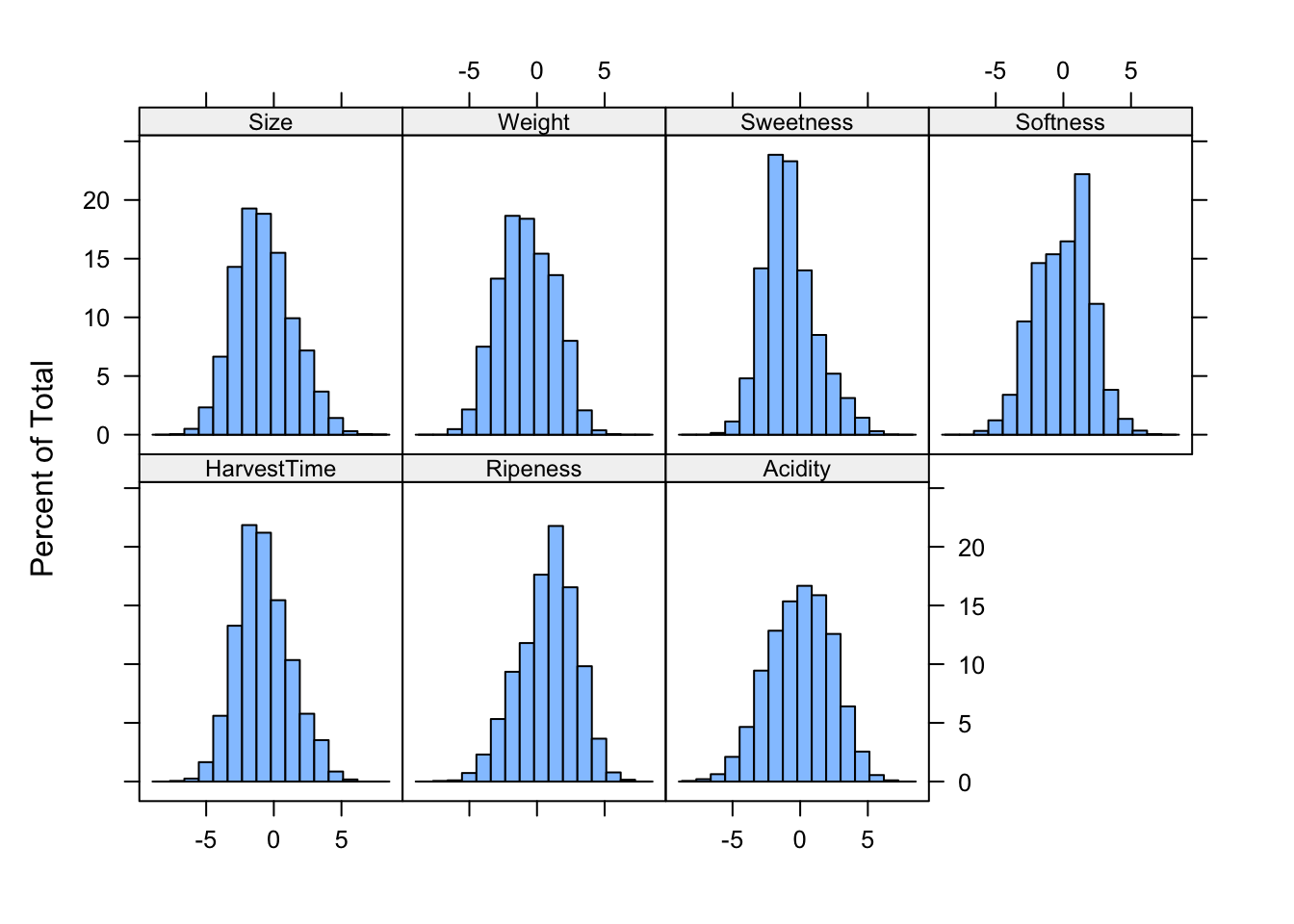
The data for this example can be found on kaggle and comprises observations on the quality of bananas (“Good”, “Bad”) and seven attributes (Figure 20.1). The attributes are normalized although it is not clear how this was done. There are 4,000 training observations and 4,000 testing observations in separate data sets.
Figure 20.1: Histograms of banana quality attributes (training data)
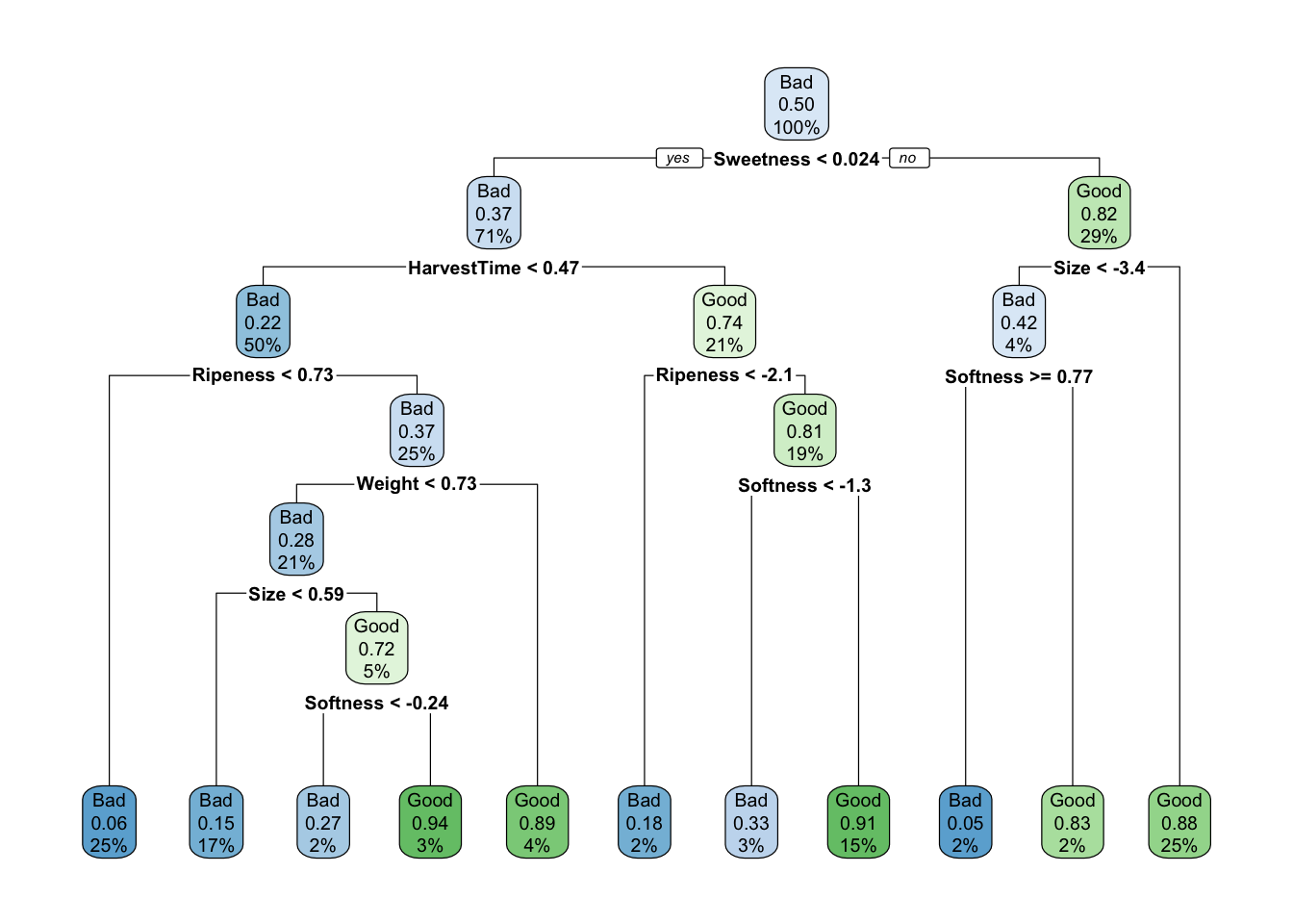
We first build a regular classification tree for the training data and compute its confusion matrix for the test data. The tree is grown with the tree::tree function and its complexity is cross-validated (10-fold) based on the misclassification rate.
As mentioned in Chapter 17, rpart performs cross-validation as part of tree construction, so no further pruning is necessary and the tree can be used to predict the test data.
Confusion Matrix and Statistics

          Reference
Prediction  Bad Good
      Bad  1723  240
      Good  271 1766

               Accuracy : 0.8722
                 95% CI : (0.8615, 0.8824)
    No Information Rate : 0.5015
    P-Value [Acc > NIR] : <2e-16

                  Kappa : 0.7445

 Mcnemar's Test P-Value : 0.1845

            Sensitivity : 0.8641
            Specificity : 0.8804
         Pos Pred Value : 0.8777
         Neg Pred Value : 0.8670
             Prevalence : 0.4985
         Detection Rate : 0.4308
   Detection Prevalence : 0.4908
      Balanced Accuracy : 0.8722

       'Positive' Class : Bad
The decision tree achieves an accuracy of 87.225% on the test data.
To apply bagging we use the randomForest function in the package by the same name. As we will see shortly, bagging is a special case of a random forest where the mtry parameter is set to the number of input variables, here 7. By default, randomForest performs \(B=500\) bootstrap samples, that is, it builds \(500\) trees.
Call:
randomForest(formula = Quality ~ ., data = ban_train, xtest = ban_test[, -8], ytest = ban_test[, 8], mtry = 7, importance = TRUE)
Type of random forest: classification
Number of trees: 500
No. of variables tried at each split: 7
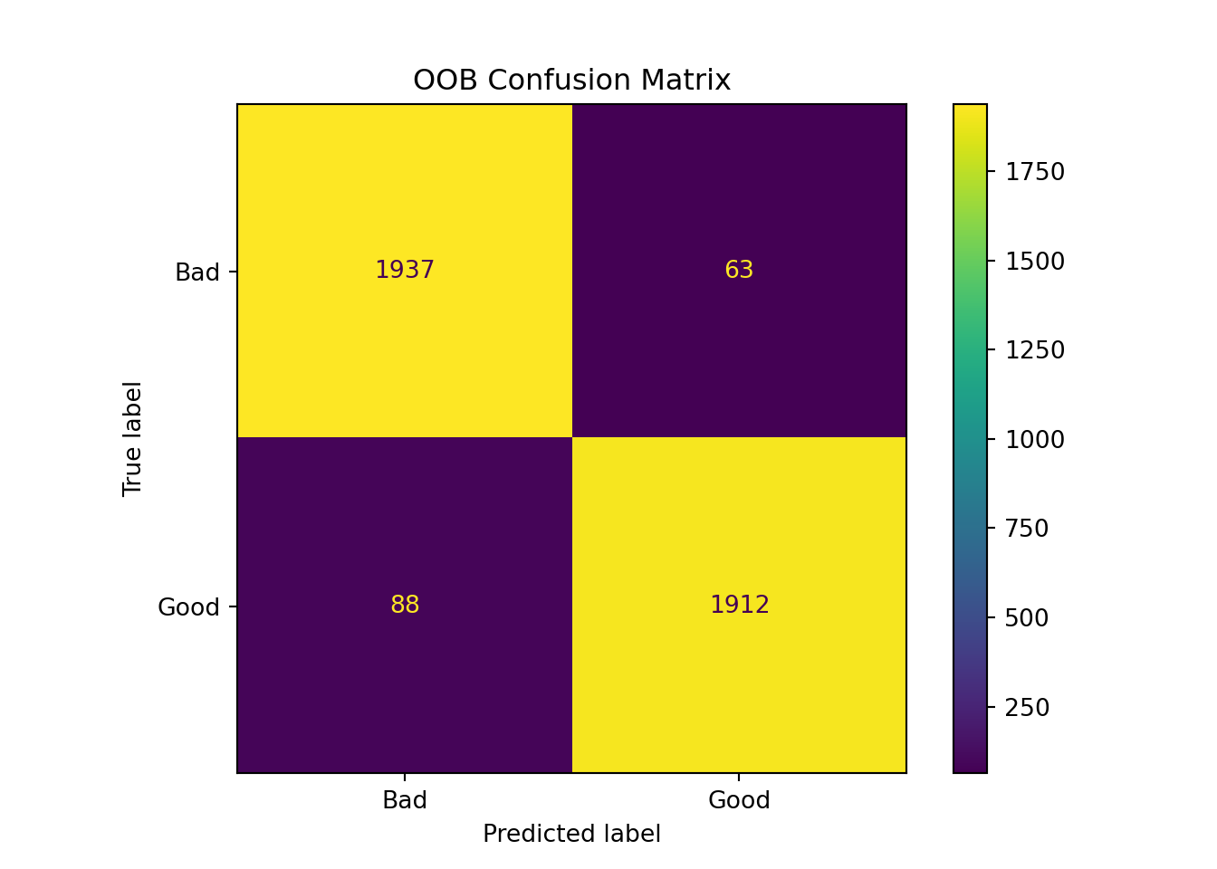
OOB estimate of error rate: 3.88%
Confusion matrix:
Bad Good class.error
Bad 1933 67 0.0335
Good 88 1912 0.0440
Test set error rate: 3.35%
Confusion matrix:
Bad Good class.error
Bad 1929 65 0.03259779
Good 69 1937 0.03439681
When a test set is specified, randomForest returns two types of predicted values. bag.ban$predicted are the out-of-bag predictions. Each observation is out-of-bag in about 1/3 of the trees built. The majority vote across the \(B/3\) classifications is the out-of-bag prediction for that observation. The predicted values based on the test data set are stored in bag.ban$test$predicted. Each observation in the test data set is passed through the 500 trees—the majority vote of the predicted quality is the overall prediction for that observation.
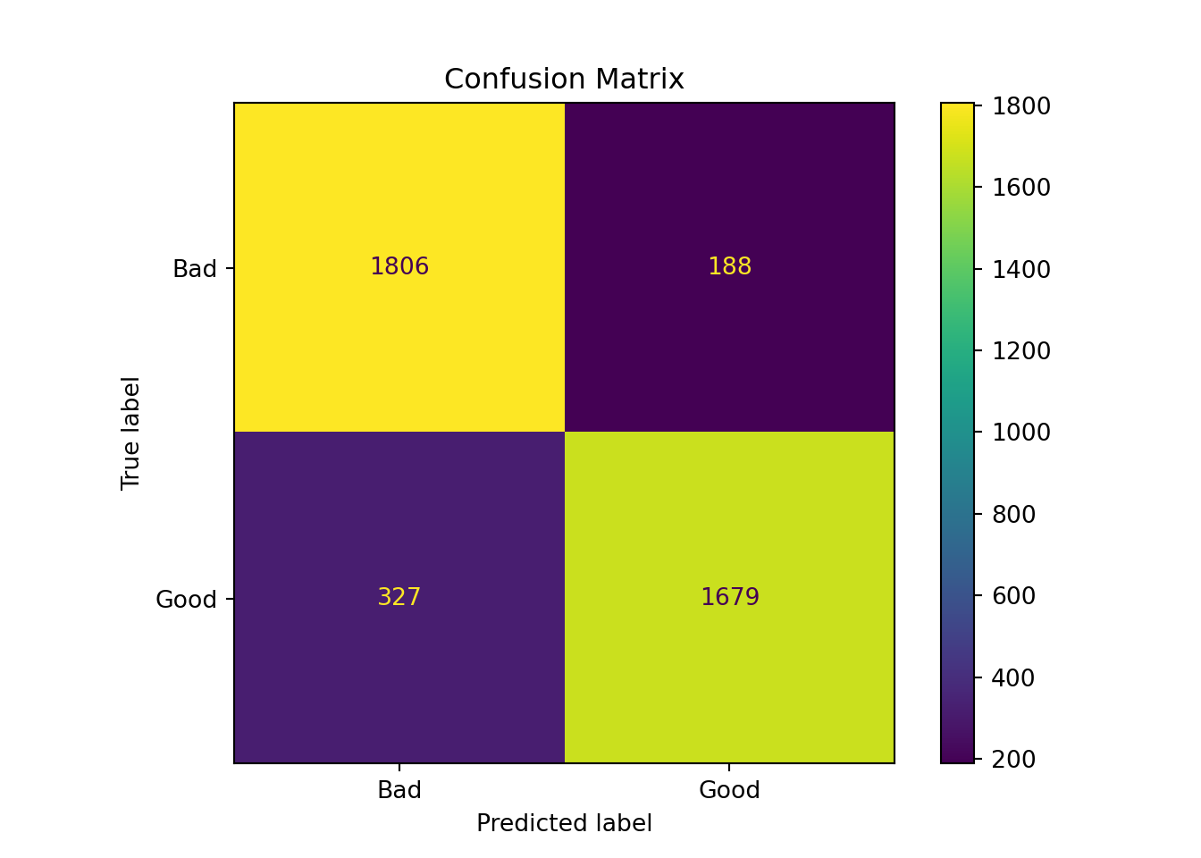
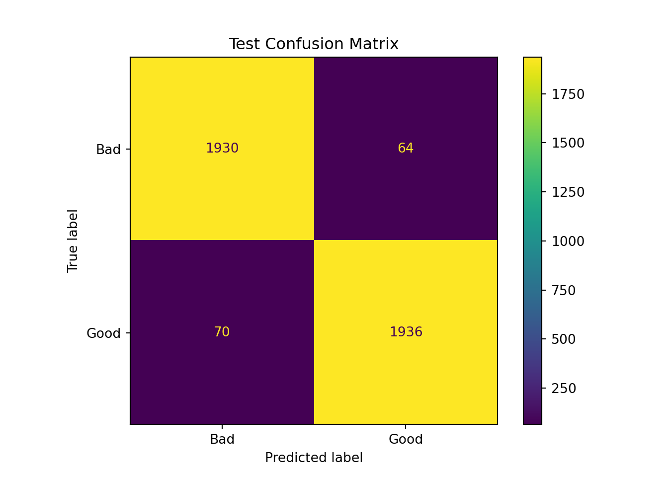
The confusion matrices shown by randomForest can be reconstructed as follows:
Confusion Matrix and Statistics

          Reference
Prediction  Bad Good
      Bad  1929   69
      Good   65 1937

               Accuracy : 0.9665
                 95% CI : (0.9604, 0.9719)
    No Information Rate : 0.5015
    P-Value [Acc > NIR] : <2e-16

                  Kappa : 0.933

 Mcnemar's Test P-Value : 0.7955

            Sensitivity : 0.9674
            Specificity : 0.9656
         Pos Pred Value : 0.9655
         Neg Pred Value : 0.9675
             Prevalence : 0.4985
         Detection Rate : 0.4823
   Detection Prevalence : 0.4995
      Balanced Accuracy : 0.9665

       'Positive' Class : Bad
The accuracy of the decision tree has increased from 87.225% for the single tree to 96.65% through bagging.
import duckdbcon = duckdb.connect("ads.ddb", read_only=True)ban_train = con.execute("SELECT * FROM banana_train").df()ban_test = con.execute("SELECT * FROM banana_test").df()con.close()
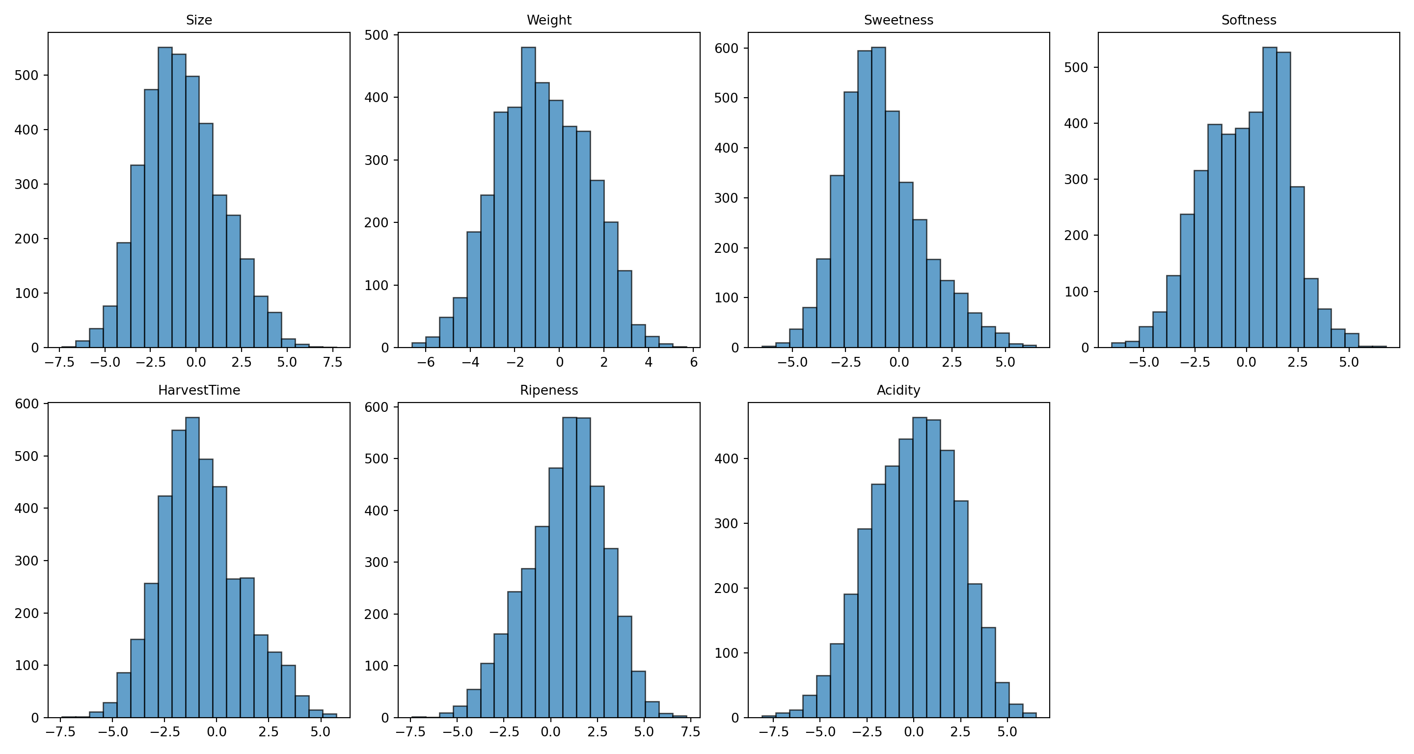
import matplotlib.pyplot as plt# Convert Quality to categoricalban_train['Quality'] = ban_train['Quality'].astype('category')ban_test['Quality'] = ban_test['Quality'].astype('category')# Create histograms fig, axes = plt.subplots(2, 4, figsize=(15, 8))axes = axes.flatten()columns = ['Size', 'Weight', 'Sweetness', 'Softness', 'HarvestTime', 'Ripeness', 'Acidity']for i, col inenumerate(columns):if i <len(axes): axes[i].hist(ban_train[col], bins=20, alpha=0.7, edgecolor='black') axes[i].set_title(col, fontsize=10) axes[i].set_xlabel('')# Hide the last empty subplotiflen(columns) <len(axes): axes[-1].set_visible(False)plt.tight_layout()plt.show()
Figure 20.2: Histograms of banana quality attributes (training data)
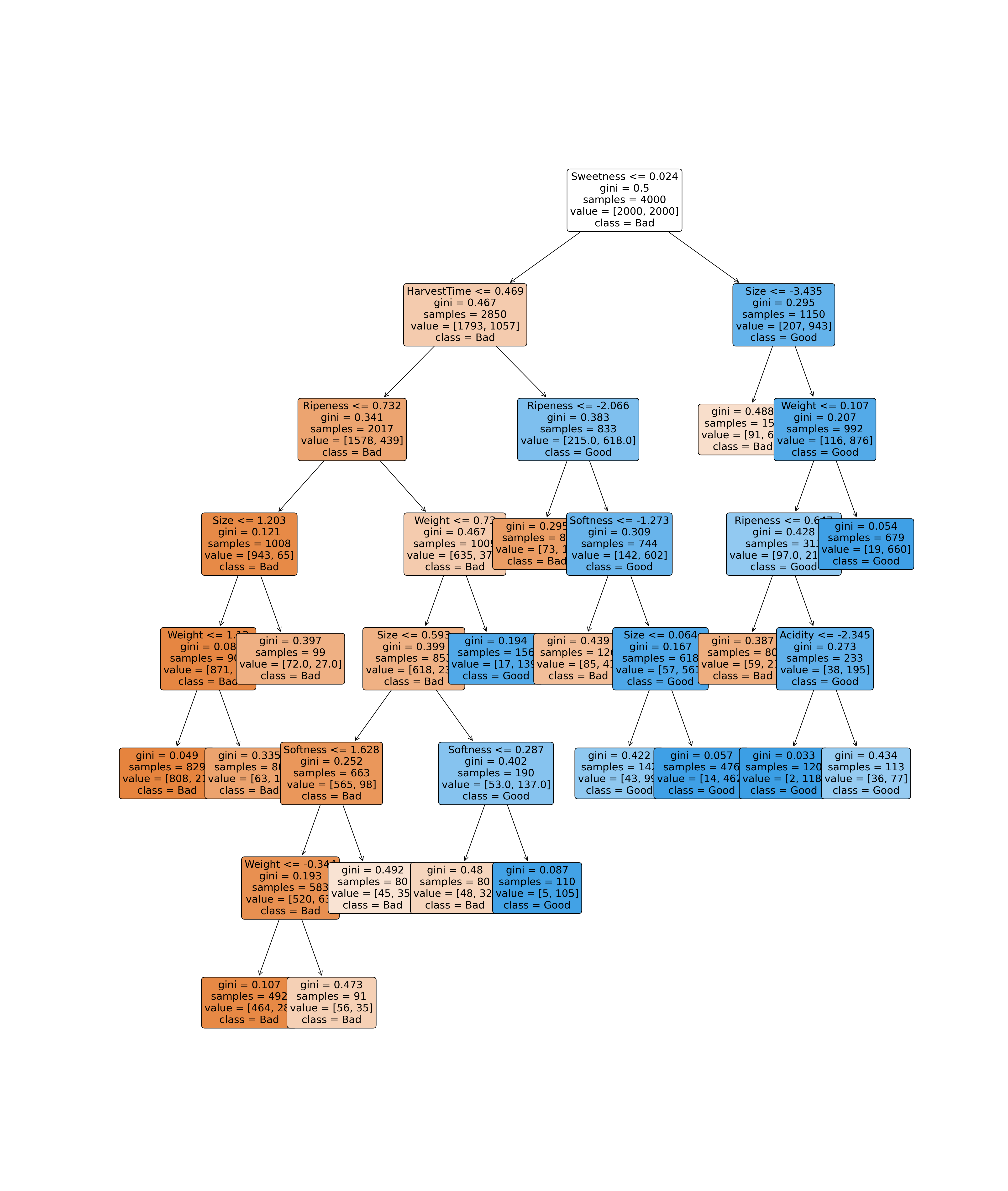
We first build a regular classification tree for the training data and compute its confusion matrix for the test data. The tree is grown with the sklearn function DecisionTreeClassifierand its complexity is cross-validated (10-fold) based on the misclassification rate.
from sklearn.tree import DecisionTreeClassifier, plot_treefrom sklearn.model_selection import cross_val_scorefrom sklearn.metrics import confusion_matrix, classification_report, ConfusionMatrixDisplay, accuracy_scorefeature_columns = ['Size', 'Weight', 'Sweetness', 'Softness', 'HarvestTime', 'Ripeness', 'Acidity']X_train = ban_train[feature_columns]y_train = ban_train['Quality']X_test = ban_test[feature_columns]y_test = ban_test['Quality']#Setting value for minimum samples per leafmin_samples =80# Create and fit decision treetree_ban = DecisionTreeClassifier(random_state=123, min_samples_leaf = min_samples)tree_ban.fit(X_train, y_train)
In a Jupyter environment, please rerun this cell to show the HTML representation or trust the notebook. On GitHub, the HTML representation is unable to render, please try loading this page with nbviewer.org.
# Calculate residual mean deviance and misclassification error ratey_train_pred = tree_ban.predict(X_train)train_accuracy = np.mean(y_train_pred == y_train)def print_tree_info(tree, accuracy): n_nodes = tree.tree_.node_count misclassification_rate =1- accuracyprint("Tree Summary")print(f"Total nodes: {n_nodes}")print(f"Number of leaves: {tree.get_n_leaves()}")print(f"Tree depth: {tree_ban.get_depth()}")print(f"Misclassification error rate: {misclassification_rate:.4f}")print(f"Accuracy: {accuracy:.4f}")print("\nFeature importance:")for name, imp inzip(tree.feature_names_in_, tree.feature_importances_):if imp >0: # Only show features that were usedprint(f"{name}: {imp:.3f}")print_tree_info(tree_ban, train_accuracy)
Tree Summary
Total nodes: 59
Number of leaves: 30
Tree depth: 10
Misclassification error rate: 0.1190
Accuracy: 0.8810

Feature importance:
Size: 0.136
Weight: 0.118
Sweetness: 0.251
Softness: 0.090
HarvestTime: 0.245
Ripeness: 0.149
Acidity: 0.011
# Cross-validation for optimal tree size (pruning)np.random.seed(123)max_leaf_nodes_range =range(2, 30)cv_scores = []for max_leaf_nodes in max_leaf_nodes_range: tree_temp = DecisionTreeClassifier(max_leaf_nodes=max_leaf_nodes, min_samples_leaf = min_samples, random_state=123) scores = cross_val_score(tree_temp, X_train, y_train, cv=10, scoring='accuracy') cv_scores.append(scores.mean())optimal_leaves = max_leaf_nodes_range[np.argmax(cv_scores)]print(f"Optimal tree size after pruning: {optimal_leaves} leaves")
Optimal tree size after pruning: 18 leaves
Based on the cross validation, a reduction in tree size provides better results. A tree will be fit with the optimal number of leaf nodes and used to make predictions with the test data.
In a Jupyter environment, please rerun this cell to show the HTML representation or trust the notebook. On GitHub, the HTML representation is unable to render, please try loading this page with nbviewer.org.
The decision tree achieves an accuracy of 87.1% on the test data.
To apply bagging we use the RandomForestClassifier function in the sklearn.ensemble module. As we will see shortly, bagging is a special case of a random forest where the max_features parameter is set to the number of input variables, here 7. To specify \(B=500\) bootstrap samples, we set n_estimators to 500. That is, it builds \(500\) trees.
from sklearn.ensemble import RandomForestClassifier# Set random seed for reproducibilitynp.random.seed(6543)# Create and fit the bagging model bag_ban = RandomForestClassifier( n_estimators=500, max_features=7, random_state=6543, bootstrap=True, oob_score=True)# Fit the modelbag_ban.fit(X_train, y_train)
In a Jupyter environment, please rerun this cell to show the HTML representation or trust the notebook. On GitHub, the HTML representation is unable to render, please try loading this page with nbviewer.org.
# Access OOB decision function for array of labeled OOB predictionsoob_proportions = bag_ban.oob_decision_function_oob_predictions = np.argmax(oob_proportions, axis=1)oob_predictions_label = pd.DataFrame(["Good"if item ==1else"Bad"for item in oob_predictions])# Obtain model predictions on the test datatest_predictions = bag_ban.predict(X_test)trees = bag_ban.n_estimatorsoob_score = bag_ban.oob_score_accuracy = accuracy_score(y_test, test_predictions)def bag_mod_sum (trees, oob_score, accuracy):# Print model summaryprint("Bagging Model Summary:")print(f"Number of trees: {trees}")print(f"OOB Score: {oob_score:.4f}")print(f"Test Accuracy: {accuracy:.4f}")bag_mod_sum (trees, oob_score, accuracy)
Bagging Model Summary:
Number of trees: 500
OOB Score: 0.9623
Test Accuracy: 0.9665
When oob_score is set to TRUE, RandomForestClassifier returns out-of-bag prediction proportions by class, bag_ban.oob_decision_function_. Each training observation is out-of-bag in about 1/3 of the trees built. The proportions are based on votes across the \(B/3\) classifications. The out-of-bag predicted quality is the one with the majority votes, and, therefore, the highest proportion of votes, for that observation.
The predicted values for the test data set are determined using the predict function. Each observation in the test data set is passed through the 500 trees—the majority vote of the predicted quality is the overall prediction for that observation.
Test accuracy: 0.9665
Test Sensitivity : 0.967904
Test Specificity : 0.965105
'Positive' Class: Bad
The accuracy of the decision tree has increased from 87.1% for the single tree to 96.65% through bagging.
As with all ensemble methods, interpretability of the results suffers when methods are combined. Decision trees are intrinsically interpretable and among the most easily understood algorithms.
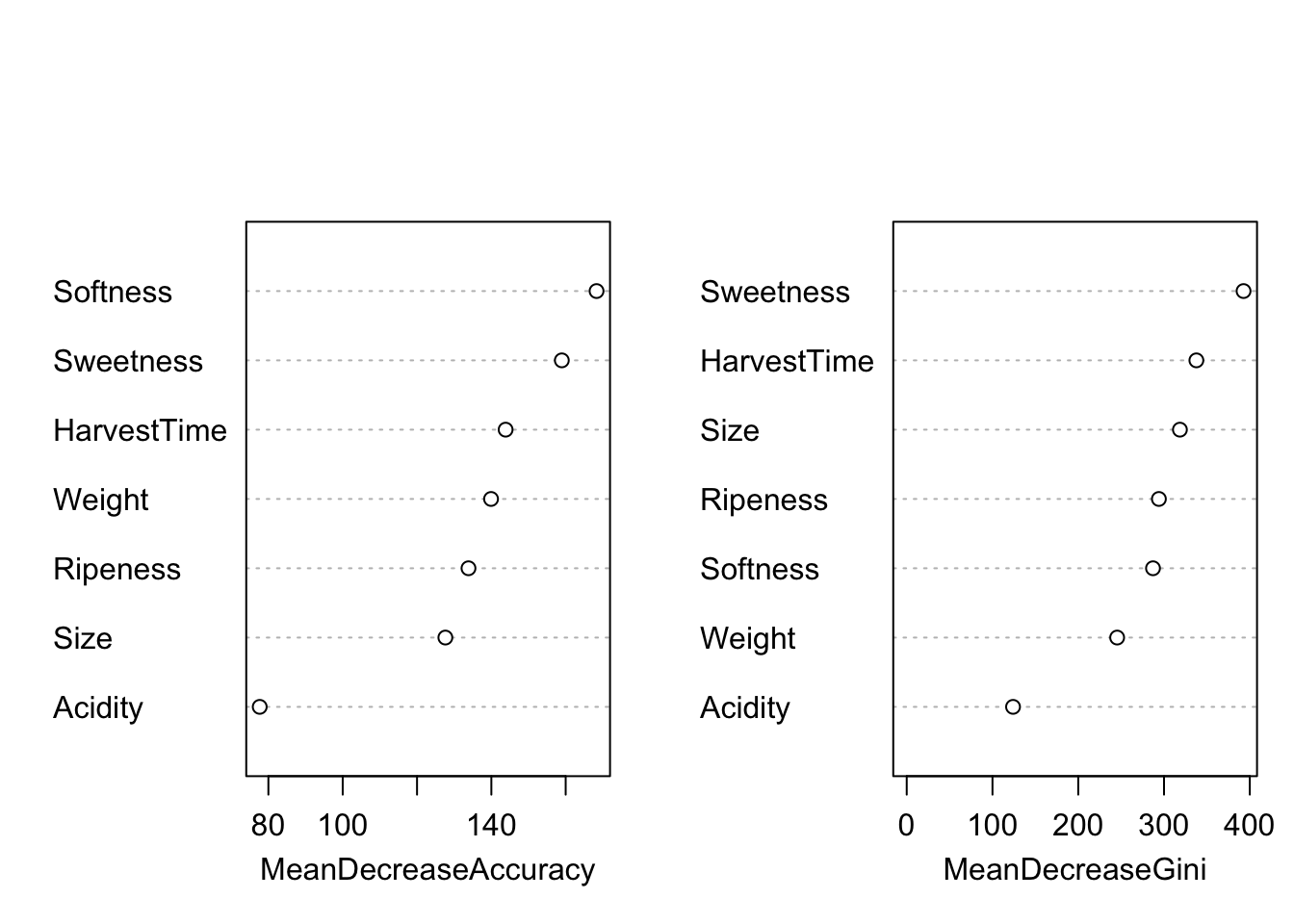
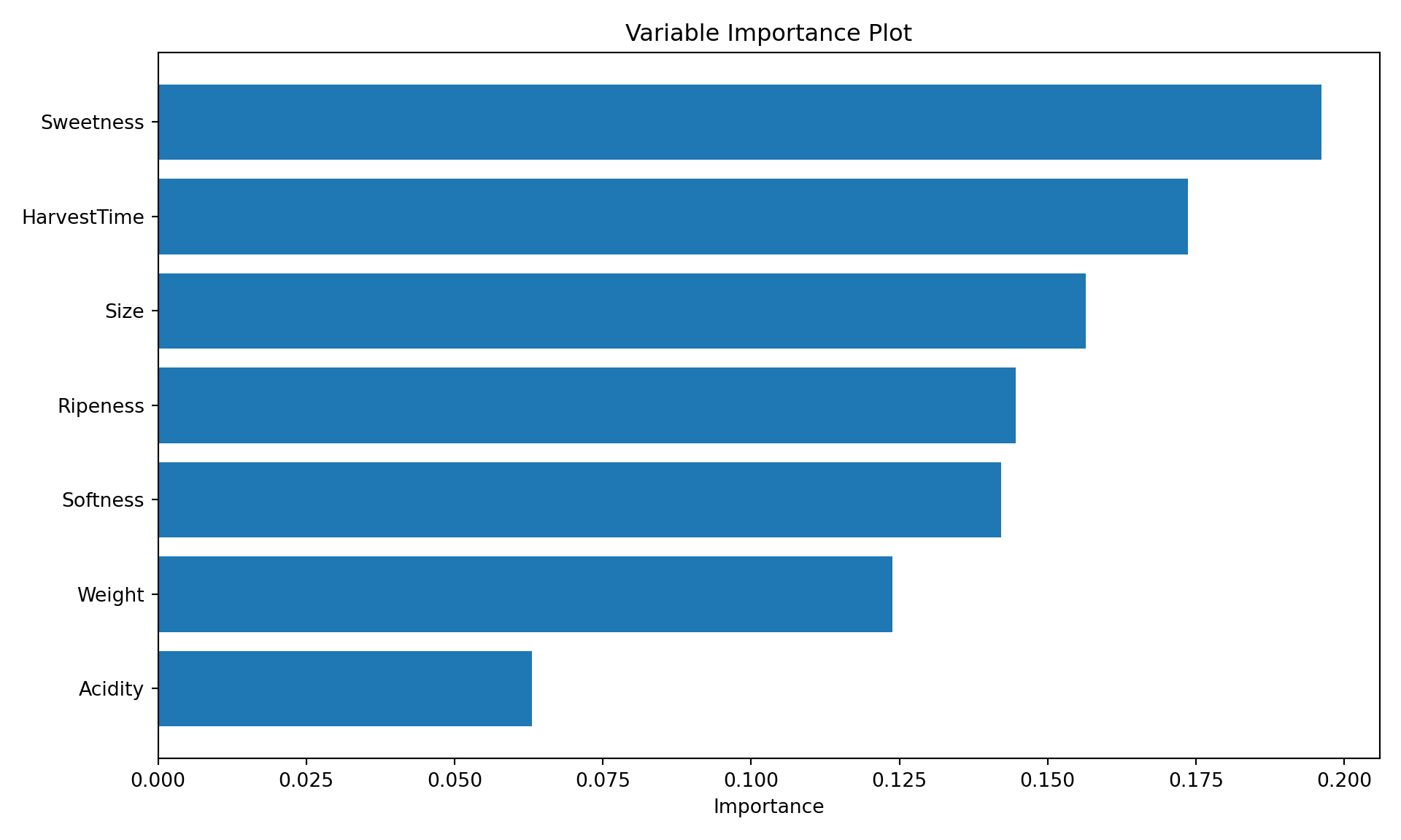
With bagged trees we lose this interpretability; instead of a single tree the decision now depends on many trees and cannot be visualized in the same way. To help with the interpretation of bagged trees, the importance of the features can be calculated in various ways. One technique uses the Gini index, a measure of the node purity, another looks at the decrease in accuracy when the variable is permuted in the out-of-bag samples. Permutation breaks the relationship between the values of the variable and the target variable. A variable that changes the accuracy greatly when its values are permuted is an important variable for the tree.
Figure 20.6: Variable importance plots for bagged trees.
Bagging is a powerful method to improve accuracy. In Breiman’s words:
Bagging goes a ways toward making a silk purse out of a sow’s ear, especially if the sow’s ear is twitchy. […] What one loses, with the trees, is a simple and interpretable structure.
What one gains is increased accuracy.
20.4 Random Forests
Are there any other downsides to bagging, besides a loss of interpretability and increased computational burden? Not really, but another issue deserves consideration: bootstrap samples are highly correlated. Two thirds of the observations are in the bootstrap samples, making the data sets similar to each other. An input variable that dominates the model will tend to be the first variable on which the tree is split, leading to similar trees. This reduces the variability of the trees and reduces the effectiveness of the ensemble.
How can we make the trees more volatile? Breiman (2001) advanced the concept of bagged trees through the introduction of random forests. The key innovation that leads from bagged trees to random forests is that not all input variables are considered at each split of the tree. Instead, only a randomly selected set of predictors is considered, the set changes from split to split. The random split introduces more variability and allows non-dominant input variables to participate.
In other aspects, random forests are constructed in the same way as bagged trees introduced in Section 20.3: \(B\) trees are built based on \(B\) bootstrap samples, the trees are built deep and not pruned.
Fitting a random forest instead of bagging trees is simple based on the previous R code. Simply specify a value for the mtry parameter that is smaller than the number of input variables. By default, randomForest chooses \(p/3\) candidate inputs at each split in regression trees and \(\sqrt{p}\) candidate inputs in classification trees.
set.seed(6543)rf.ban <-randomForest(Quality ~ . , data =ban_train, xtest=ban_test[,-8],ytest=ban_test[, 8])rf.ban
Call:
 randomForest(formula = Quality ~ ., data = ban_train, xtest = ban_test[,      -8], ytest = ban_test[, 8])
               Type of random forest: classification
                     Number of trees: 500
No. of variables tried at each split: 2

        OOB estimate of  error rate: 3.3%
Confusion matrix:
      Bad Good class.error
Bad  1944   56       0.028
Good   76 1924       0.038
                Test set error rate: 3.15%
Confusion matrix:
      Bad Good class.error
Bad  1928   66  0.03309930
Good   60 1946  0.02991027
Only two of the seven inputs are considered at each split in the random forest compared to the bagged trees. The accuracy improves slightly from 96.65% to 96.85%.
Fitting a random forest instead of bagging trees is simple based on the previous code. Simply specify a value for the max_features parameter that is smaller than the number of input variables. By default, RandomForestRegressor chooses \(p\) candidate inputs at each split in regression trees, and RandomForestClassifer chooses \(\sqrt{p}\) candidate inputs in classification trees.
# Standard Random Forest (equivalent to rf.ban)np.random.seed(6543)rf_ban = RandomForestClassifier( n_estimators=500, max_features='sqrt', random_state=6543, bootstrap=True, oob_score=True)# Fit the standard random forestrf_ban.fit(X_train, y_train)
In a Jupyter environment, please rerun this cell to show the HTML representation or trust the notebook. On GitHub, the HTML representation is unable to render, please try loading this page with nbviewer.org.
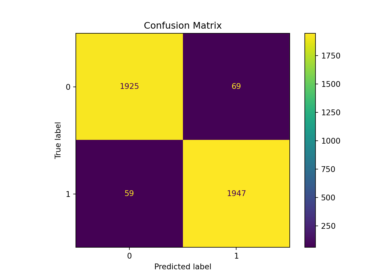
# Print standard RF resultsdef rf_mod_sum(rf_fit, x, y):# Make predictions rf_predictions = rf_fit.predict(x)print("Random Forest Model Summary:")print(f"Number of trees: {rf_fit.n_estimators}")print(f"Max features per split: 2")print(f"OOB Score: {rf_fit.oob_score_:.4f}")print(f"Test Accuracy: {accuracy_score(y, rf_predictions):.4f}") cm = confusion_matrix(y, rf_predictions) disp = ConfusionMatrixDisplay(confusion_matrix= cm) disp.plot() disp.ax_.set_title("Confusion Matrix") plt.show()rf_mod_sum(rf_ban, X_test, y_test)
Random Forest Model Summary:
Number of trees: 500
Max features per split: 2
OOB Score: 0.9673
Test Accuracy: 0.9680
Only two of the seven inputs are considered at each split in the random forest compared to the bagged trees. The accuracy improves slightly from 96.65% to 96.80%.
It might seem counterintuitive that one can achieve a greater accuracy by “ignoring” five out of the seven input variables at each split. It turns out that the results are fairly insensitive to the number of inputs considered at each split. The important point is that not all inputs are considered at each split. In that case, one might as well choose a small number to speed up the computations.
Bagged trees and random forests are easily parallelized, the \(B\) trees can be trained independently. This is different from other ensemble techniques, for example, boosting that builds the ensemble sequentially. Another advantage of bootstrap-based methods is that they do not overfit. Increasing \(B\), the number of bootstrap samples, simply increases the number of trees but does not change the model complexity.
Cross-validation is not necessary with bootstrap-based methods because the out-of-bag error can be computed from the observations not in a particular bootstrap sample.
Using a random selection of inputs at each split is one manifestation of “random” in random forests. Other variations of random forests take random linear combinations of inputs, randomizing the outputs in the training data or random set of weights. The important idea is to inject randomness into the system to create diversity.
Random forests excel at reducing variability and there is some evidence that they also reduce bias. Breiman (2001) mentions that the mechanism by which forests reduce bias is not obvious. The bootstrap mechanism is inherently focused on reducing variability. A different class of ensemble methods was developed to attack both bias and variance simultaneously. In contrast to the random forest, these boosting techniques are based on sequentially changing the training data set or the model (Chapter 21).
A yet completely different approach is taken by Bayesian Model Averaging (BMA). In many situations there is no one clear winning model but a neighborhood of models that deserve consideration. Picking a single winner then seems not justified. Providing interpretations of a large number of models is also not advised. BMA combines many models to contribute to an overall prediction according to their proximity to the best-performing model (Chapter 22).