Classification methods based on support vectors were introduced in the 1990s and made a big splash. Their approach to solving classification problems was novel and intuitive, they showed excellent performance, and worked well in high dimensions even when \(p \gg n\). The approach was refreshing and distinctly different from traditional approaches such as logistic regression or linear discriminant analysis.
The performance of support vector methods, especially support vector machines (SVM, see Section 15.4 below) was so impressive that the technique became an off-the-shelf standard classifier for many data scientists. Much so as (extreme) gradient boosting has become an off-the-shelf default method for many data scientists solving regression problems. Support vector machines have since been extended to regression problems; we consider them primarily for classification here.
How impressive is the performance of support vector methods? Consider the following example, classifying bananas into “Good” and “Bad” quality based on fruit attributes such as size, weight, sweetness, ripeness, etc. You can find the data set for this analysis on kaggle.
Example
Example: Banana Quality
4,000 observations are in the training set, 4,000 observations are in the test data set.
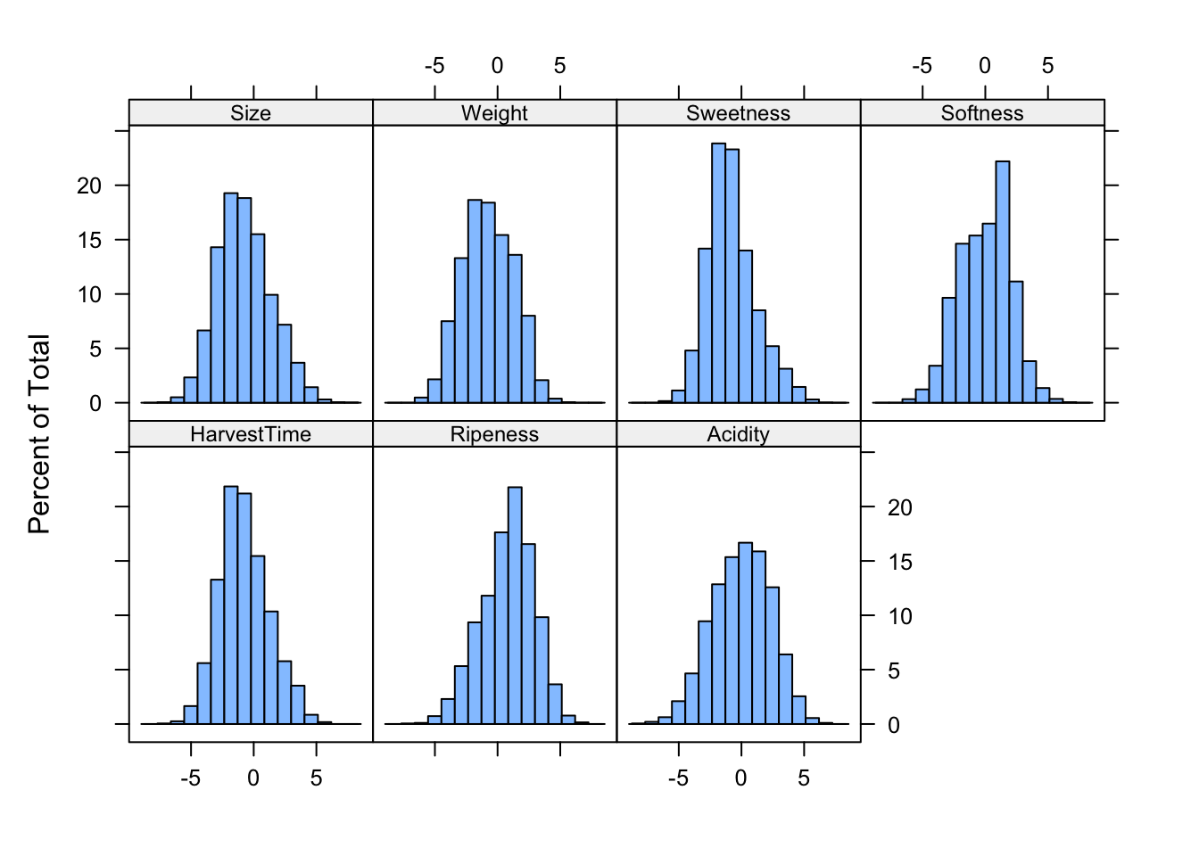
Figure 15.1: Histogram of attributes in banana training data set.
The following statements use the e1071::svm function to train a support vector machine on the training data and compute the confusion matrix for the test data. Because the data are already scaled (see Figure 15.1), we set scale=FALSE. Otherwise, this is the default SVM analysis.
Confusion Matrix and Statistics

          Reference
Prediction  Bad Good
      Bad  1957   44
      Good   37 1962

               Accuracy : 0.9798
                 95% CI : (0.9749, 0.9839)
    No Information Rate : 0.5015
    P-Value [Acc > NIR] : <2e-16

                  Kappa : 0.9595

 Mcnemar's Test P-Value : 0.505

            Sensitivity : 0.9781
            Specificity : 0.9814
         Pos Pred Value : 0.9815
         Neg Pred Value : 0.9780
             Prevalence : 0.5015
         Detection Rate : 0.4905
   Detection Prevalence : 0.4998
      Balanced Accuracy : 0.9798

       'Positive' Class : Good
This out-of-the-box analysis achieves an impressive 97.975% accuracy on the test data set. With tuning of hyperparameters (see Section 15.4), this accuracy can be increased even further. The sensitivity and specificity of the model are also impressive. For comparisons, an out-of-the-box logistic regression achieves 88.1% accuracy, a finely grown and pruned decision tree achieves 89.5% accuracy.
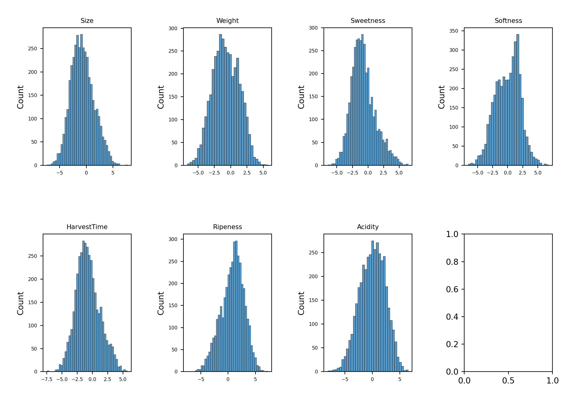
Figure 15.2 displays histograms for the fruit attributes in the training data.
import duckdbcon = duckdb.connect(database="ads.ddb", read_only=True)ban_train = con.sql("SELECT * FROM banana_train").df()ban_test = con.sql("SELECT * FROM banana_test").df()con.close()ban_train['Quality'] = ban_train['Quality'].astype('category')ban_test['Quality'] = ban_test['Quality'].astype('category')
import pandas as pdimport matplotlib.pyplot as pltimport seaborn as snsfig, axes = plt.subplots(nrows=2, ncols=4, figsize=(10, 7))fig.tight_layout(pad=3.0)# Variables to plotvariables = ['Size', 'Weight', 'Sweetness', 'Softness', 'HarvestTime', 'Ripeness', 'Acidity']for i, var inenumerate(variables): row = (i >=4)*1 sns.histplot(data=ban_train, x=var, ax=axes[row, i %4]) axes[row, i %4].set_title(var, fontsize=8) axes[row, i %4].tick_params(labelsize=6) axes[row, i %4].set_xlabel('')# Adjust layoutplt.subplots_adjust(hspace=0.5)plt.show()
Figure 15.2: Histogram of attributes in banana training data set.
The following statements use the svm function of sklearn to train a support vector machine on the training data and compute the confusion matrix for the test data. Because the data are already scaled (see Figure 15.2), we set scale=FALSE. Otherwise, this is the default SVM analysis.
In a Jupyter environment, please rerun this cell to show the HTML representation or trust the notebook. On GitHub, the HTML representation is unable to render, please try loading this page with nbviewer.org.
SVC()
pred = ban_svm.predict(X_test)cm = confusion_matrix(y_test, pred)print("Confusion Matrix:")
Confusion Matrix:
print(cm)
[[1958   36]
 [  46 1960]]
# Create classification report (similar to confusionMatrix in R)positive_class ="Good"# Assuming "Good" is one of your quality levelstarget_names = ban_test['Quality'].unique()# Calculate metrics similar to confusionMatrix from caretreport = classification_report(y_test, pred, target_names=target_names, output_dict=True)print("\nClassification Report:")
This out-of-the-box analysis achieves an impressive 98% accuracy on the test data set. With tuning of hyperparameters (see Section 15.4), this accuracy can be increased even further. The sensitivity and specificity of the model are also impressive. For comparisons, an out-of-the-box logistic regression achieves 88.1% accuracy, a finely grown and pruned decision tree achieves 89.5% accuracy.
What is a Support Vector
The name of this family of methods stems from classification rules that are based on a subset of the observations, these observations are called the support vectors of the classifier. A support vector classifier with 10 support vectors, for example, uses the data from 10 observations to construct the classification rule, even if the training data contains 1 million observations. The number of support vectors is not a parameter you set in advance, however. Rather, you specify the constraints imposed on the classifier through other hyperparameters—such as the cost of a misclassification and the kernel function—and the number of support vectors is the result of training the classifier.
Types of Support Vector Methods
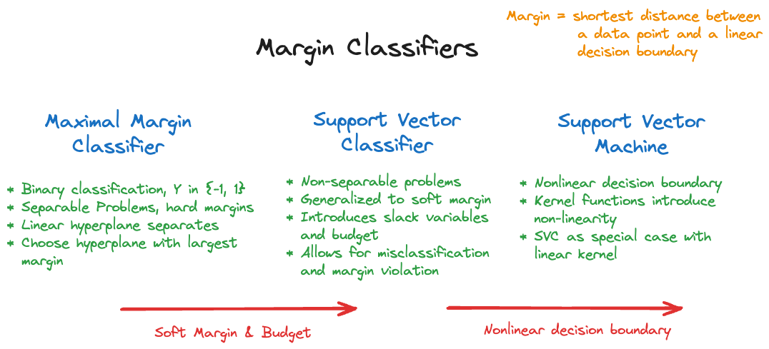
Chapter 9 of James et al. (2021) provides a great introduction into the support-vector based methods and we follow their general flow here. To arrive at support vector machines it is helpful to develop them from simpler methods, the maximal margin classifier and the support vector classifier (Figure 15.3).
Figure 15.3: The family of support vector-based classifiers.
The maximal margin classifier (MMC) is a rather simple classifier for separable cases. Suppose you are dealing with a two-category problem. This is said to be separable if you can find a classification rule that assigns every observation in the training data without error to one of the two classes.
Although intuitive, MMC is not a strong contender, most data are not completely separable. The support vector classifier (SVC) improves over the MMC by permitting a gray area of misclassification. It is OK to have a certain misclassification rate on the training data, if it improves generalizability to new observations. Finally, the support vector machine (SVM) generalizes the linear decision rule of the SVC to nonlinear decision boundaries by introducing kernel functions. The SVC emerges as a special case of SVM with a linear kernel function.
In the remainder of the chapter we discuss the three margin classifiers for binary data. As is customary with classification models not based on regression techniques, the target variable is coded \(Y \in \{-1,1\}\), rather than \(Y \in \{0,1\}\). A side effect of this target encoding is that the classification rule uses only the sign of the predicted value. If \(Y = -1\) encodes label \(A\) and \(Y=1\) encodes label \(B\), then we predict \(A\) if \(\widehat{y} < 0\) and predict \(B\) if \(\widehat{y}> 0\).
15.2 Maximal Margin Classifier (MMC)
Suppose we have \(p\) input variables \(X_1,\cdots,X_p\). For each observation in the training data we have \([y_i, x_{i1}, \cdots, x_{ip}]^\prime = [y_i, \textbf{x}_i]\). Given a new data point for the inputs, \(\textbf{x}_0 = [x_{01}, \cdots, x_{0p}]^\prime\), should we assign it to the \(-1\) or the \(1\) category?
The MMC asks to find a hyperplane \[
h(\textbf{x}) = \beta_0 + \beta_1 x_1 + \cdots + \beta_p x_p
\] that satisfies \[
y_i h(\textbf{x}_i) = y_i \, \left ( \beta_0 + \beta_1 x_{i1} + \cdots + \beta_p x_{ip} \right )> 0\text{, } \forall i=1, \cdots, n
\] Recall that \(y_i \in \{-1,1\}\). This condition states that all training observations fall either on the right or the left side of \(h(\textbf{x})\). There are no misclassifications which would occur if \(h(\textbf{x}_i) < 0\) and \(y = 1\) or if \(h(\textbf{x}_i) > 0\) and \(y = -1\).
Once we have found \(h(\textbf{x})\), we classify \(\textbf{x}_0\) by computing \(h(\textbf{x}_0)\)\[
\widehat{y} = \left \{ \begin{array}{r l}
1 & h(\textbf{x}_0) > 0 \\ -1 & h(\textbf{x}_0) < 0
\end{array} \right .
\]
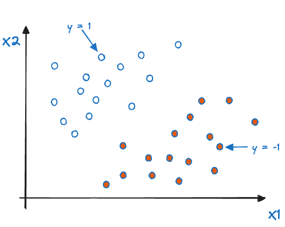
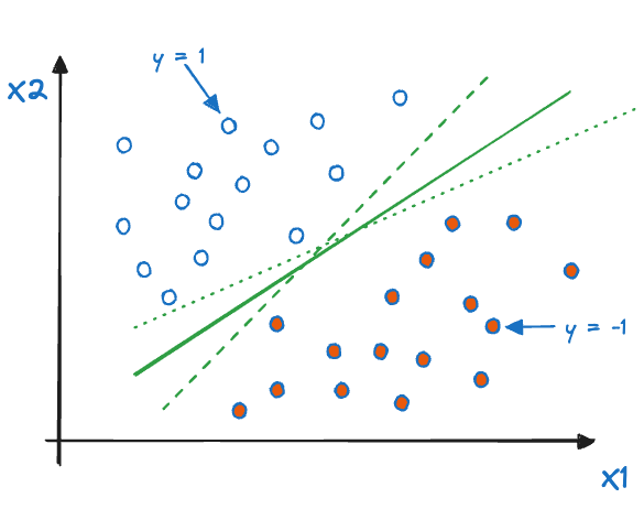
Figure 15.4 shows the basic setup for a maximal margin classifier with two inputs. The hyperplane \(h(\textbf{x}) = \beta_0 + \beta_1 x_1 + \beta_2 x_2\) in two dimensions is a line. The data are separable in the sense that we can find coefficients \(\beta_0, \beta_1, \beta_2\) so that the line carves through the figure in such a way that all points with \(y=1\) fall on one side of the line (\(h(\textbf{x}) > 0\)), and all points with \(y= -1\) fall on the other side of the line (\(h(\textbf{x}) < 0\)). For all points that lie exactly on the hyperplane, we have \(h(\textbf{x}) = 0\).
Figure 15.4: Maximal margin classifier for \(p=2\).
This problem can have more than one solution. For example, Figure 15.5 depicts three hyperplanes \(h_1(\textbf{x})\), \(h_2(\textbf{x})\), and \(h_3(\textbf{x})\) that satisfy the no-misclassification requirement. How should we define an optimal solution?
Figure 15.5: Three possible solutions for the MMC problem.
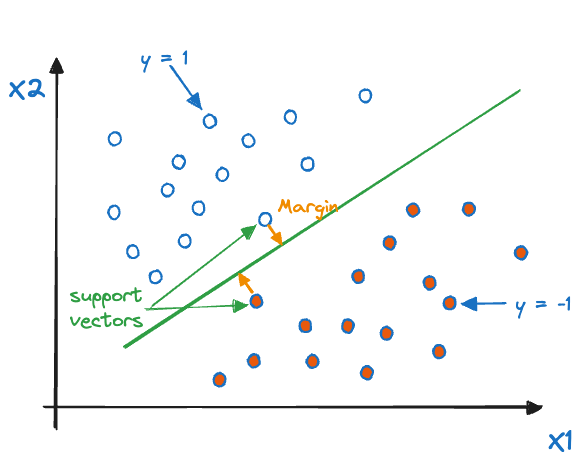
The margin of a classifier is the shortest perpendicular distance between the training observations and the hyperplane. The best solution to the problem of classifying separable observations with a linear decision boundary is to find the hyperplane that has the largest margin (the largest minimum distance between training obs and hyperplane). The rationale is that a large margin on the training data will lead to a high accuracy on the test data, if the test data are a random subset of the training data.
The observations that have the shortest distance to the hyperplane—the observations that define the margin—are called the support vectors (Figure 15.6) because they support the hyperplane as the decision boundary of the classification problem. What happens if we were to move an observation in Figure 15.6, with the caveat that the observation has to stay on the same side of the hyperplane? If the observation is not a support vector, then the hyperplane is not affected, unless the observation is moved closer to the plane than any of the support vectors. Changing the support vectors will change the hyperplane.
Figure 15.6: Example of an MMC that depends on two support vectors.
15.3 Support Vector Classifier
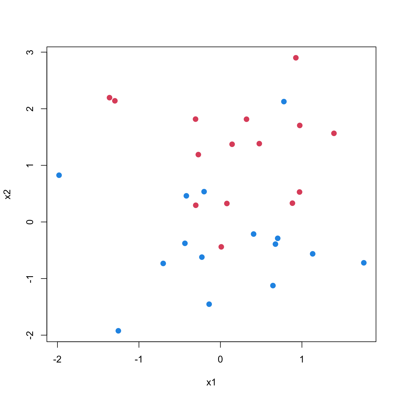
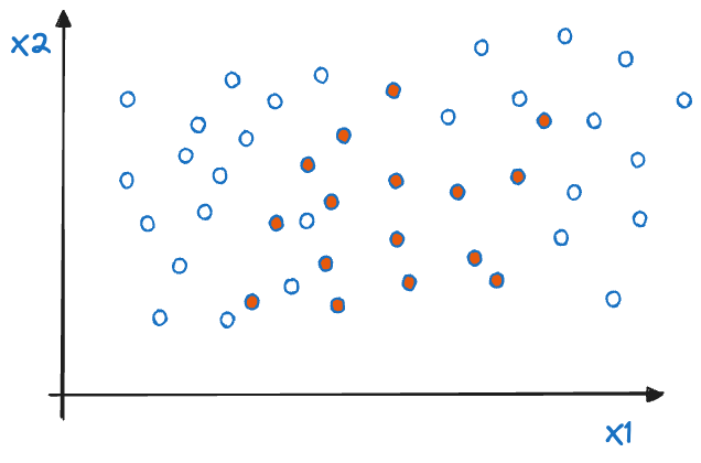
The MMC is based on a simple and intuitive idea and a solution can be found with a straightforward optimization algorithm. However, we will not consider this classifier much further, its utility lies in introducing the idea of a margin-based classifier, a linear decision boundary, and the concept of the support vector. It is not that useful in practical applications because most problems are not separable. How could we separate the points in Figure 15.7 without error by drawing a line through the plot?
Figure 15.7: A non-separable case in two dimensions
A perfect classification on the training data is also not generally desirable. It will likely lead to an overfit model that does not generalize well to new observations.
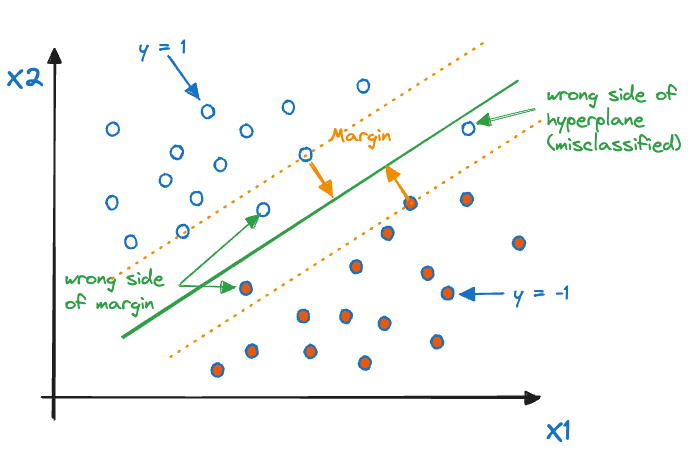
The support vector classifier (SVC) extends the MMC by finding a hyperplane that provides better classification of most observations and is more robust to individual data points (Figure 15.8).
The margin of the SVC is called a soft margin: some observations are allowed to be on the wrong side of the margin and some observations are allowed to be on the wrong side of the hyperplane (misclassified).
Figure 15.8: Support vector classifier in two dimensions.
The support vectors of the SVC are the observations that lie on the margin or lie on the wrong side of the margin for their category. As with the MMC, the decision boundary depends only on these observations. Moving any of the other observations without crossing into the margin or across the decision boundary has no effect on the optimal hyperplane.
How do we find the optimal hyperplane for the support vector classifier? One approach is to give ourselves a budget of observations that violate the margin and make sure that the chosen hyperplane does not exceed the budget. Alternatively, we can specify the cost associated with a margin violation and find the hyperplane that minimizes the overall expense.
Using the cost approach, the optimization problem that finds the SVC can be expressed as follows: \[
\begin{align*}
\mathop{\mathrm{arg\,min}}_{\boldsymbol{\beta},\boldsymbol{\epsilon}} &\, \frac12 \boldsymbol{\beta}^\prime\boldsymbol{\beta}+ C\sum_{i=1}^n \epsilon_i \\
\text{subject to } &\, y_i(\beta_0 + \beta_1x_1 + \cdots + \beta_p x_p) \ge 1-\epsilon_i \\
\epsilon_i &\ge 0, \quad i=1,\cdots,n
\end{align*}
\]
The \(\epsilon_i\) are called the slack variables, each observation is associated with one. If \(\epsilon_i = 0\), the \(i\)th observation does not violate the margin. If \(0 < \epsilon_i \le 1\), the observation violates the margin but is not misclassified. Finally, misclassified observations in the training data have \(\epsilon_i > 1\).
\(C\) is the hyperparameter representing the cost of a margin violation and is usually determined by some form of cross-validation. Choosing \(C\) is a typical bias-variance tradeoff.
\(C\) small: the cost of a margin violation is low, encouraging more violations. The resulting classifier will have a wider margin and more support vectors. This results in classifiers that are more stable, with lower variance but potentially higher bias.
\(C\) large: we have a low tolerance for margin violations. This encourages a small margin and few support vectors, resulting in classifiers that are closely fit to the training data, have low bias but potentially high variance.
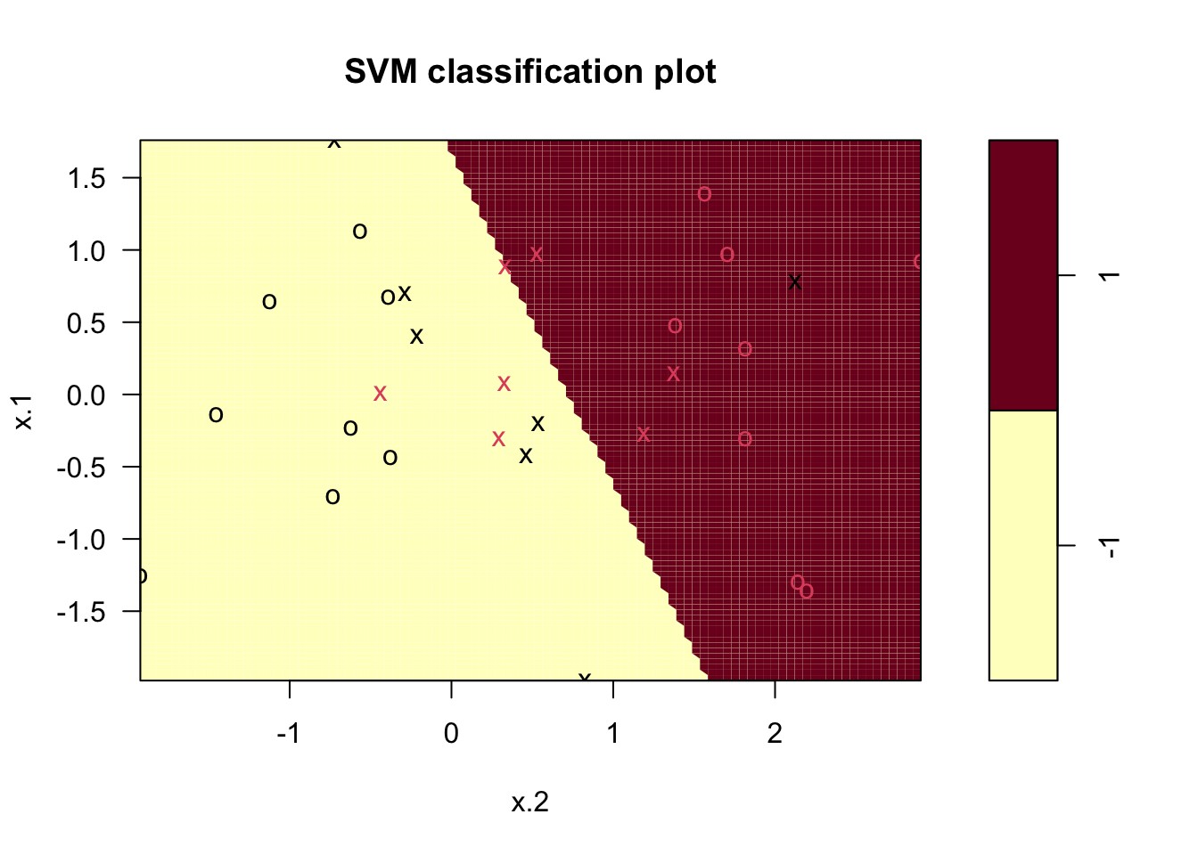
Figure 15.9 displays the decision rule for a support vector classifier fit to the data in Figure 15.7. For the particular choice of \(C\), the classification boundary depends on 14 support vectors (data points). These are shown in the plot as “x” symbols. Observations on which the hyperplane does not depend are shown as “o” symbols. You can see that some of the support vectors are on the correct side of the decision boundary and others are not. Given the chosen value of \(C\), this is the best one can achieve using a linear decision boundary for this non-separable problem.
Figure 15.9: Support vector classifier trained on data in Figure 15.7
We have not shown the code that leads to the classification plot in Figure 15.9 because the SVC turns out to be a special case of the next family of models, the support vector machines.
15.4 Support Vector Machines (SVM)
The support vector classifier is a marked improvement over the maximal margin classifier in that it can handle non-separable cases, allows cross-validation of the cost (or budget) hyperparameter, and is robust to observations that are far away from the decision boundary.
The shortcoming of the SVC is its linear decision boundary. If such a boundary applies in the case of two inputs, it means we can segment the \(x_1\)—\(x_2\) plane with a line as the classification rule. Consider the data in Figure 15.10. No linear decision boundary would slice the data to produce a good classification.
Figure 15.10: Data for which a linear decision boundary does not work well.
Just like linear regression models do not perform well if the relationship between target and inputs is nonlinear, a classifier with a linear decision rule will not classify well if the decision boundary should be nonlinear. One approach to introduce nonlinearity (in the inputs) in the regression context is to add transformations of the variables, for example, using polynomials. Similarly, we could consider revising the decision boundary in a margin classifier to include additional terms: \[
h(\textbf{x}) = \beta_0 + \beta_1 x_1 + \beta_2 x_2 + \beta_3 x_1^2 + \beta_4 x_2^2
\] But where do we stop? What is the best order of the polynomial terms, and what about the transformations \(\log(X)\) or \(\sqrt{X}\) or \(1/x\) and what about interaction terms? This could get quickly out of hand.
Support vector machines rely on what is known as the kernel trick to essentially increase the number of features, introduce nonlinearity, but without increasing numerical complexity. The principal idea is to apply a nonlinear transformation to the \(X\)-space such that a linear decision boundary is reasonable in the transformed space. In other words, find a nonlinear decision boundary in \(X\)-space as a linear decision boundary in the transformed space.
The Kernel Trick
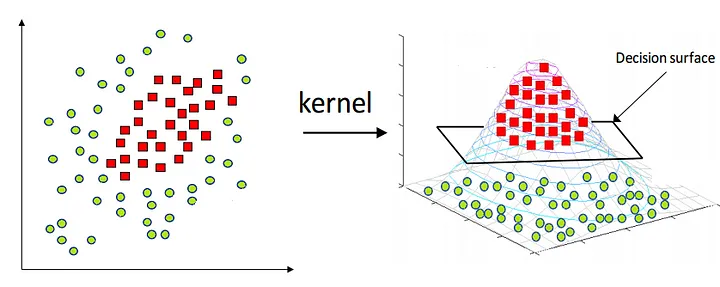
Figure 15.11 from Zhang (2018) evokes how a problem that appears not linearly separable in a lower-dimensional space becomes linearly separable in a higher-dimensional space.
Figure 15.11: A nonseparable problem in 2-D becomes linearly separable in 3-D. From Zhang (2018).
In 2-dimensional space, the linear decision boundary is a line, in 3-dimensional space the linear decision boundary (the hyperplane) is an actual plane.
The kernel trick allows us to make computations in higher-dimensional, nonlinear spaces based on only inner products of the coordinates in the original space. Wait, what?
Inner products
A kernel \(K(\textbf{x}_j,\textbf{x}_j)\) is a generalization of the inner product \[
\langle \textbf{x}_i, \textbf{x}_j \rangle = \sum_{k=1}^p x_{ik} x_{jk}
\] Instead of applying the inner product to the original coordinates \(\textbf{x}_i\) and \(\textbf{x}_j\), we first transform the coordinates. \[
K(\textbf{x}_i,\textbf{x}_j) = \langle g(\textbf{x}_i), g(\textbf{x}_j) \rangle
\] Let’s look at an example. Suppose \(\textbf{x}\) is two-dimensional, \(\textbf{x}= [x_1,x_2]\) and we define the transformations \[
\begin{align*}
g_1(\textbf{x}) &= 1 \\
g_2(\textbf{x}) &= \sqrt{2}x_1 \\
g_3(\textbf{x}) &= \sqrt{2}x_2\\
g_4(\textbf{x}) &= x_1^2 \\
g_5(\textbf{x}) &= x_2^2 \\
g_6(\textbf{x}) &= \sqrt{2}x_1 x_2
\end{align*}
\tag{15.1}\] The inner product of \(g(\textbf{x})\) with itself is then \[
g(\textbf{x})^\prime g(\textbf{x}) = 1 + 2 x_1^2 + 2 x_2^2 + x_1^4 + x_2^4 + 2x_1^2 x_2^2
\] The inner product in the transformed space includes higher-dimensional terms, without increasing the number of inputs in the calculation. That is neat, but have we gained that much? How are we to choose the transformations \(g_1(\textbf{x}),\cdots, g_m(\textbf{x})\) in a meaningful way?
Kernel functions
This is where the following result comes to the rescue. We do not need to specify the functions \(g_1(\textbf{x}),\cdots, g_m(\textbf{x})\) explicitly. Instead, we can start by choosing the kernel function \(K(\textbf{x}_i,\textbf{x}_j)\). Any valid kernel implies some transformation: \[
K(\textbf{x}_i, \textbf{x}_j) = \langle \phi(\textbf{x}_i), \phi(\textbf{x}_j) \rangle
\] for some function \(\phi()\).
Popular kernel functions in support vector machines include the following:
The quantities \(\gamma\) and \(c_0\) in these expressions are parameters of the kernel functions. They are treated as hyperparameters in training the models and often determined by a form of cross-validation.
To see the connection between choosing a kernel function and its implied transformations \(g_1(\textbf{x}), \cdots, g_m(\textbf{x})\), consider the polynomial kernel of second degree (\(d=2\)), \(c_0 = 1\) and \(\gamma = 1\). Then \[
\begin{align*}
(1+\langle [x_1, x_2], [x_1, x_2]\rangle)^2 &= \left ( 1 + x_1 x_1 + x_2 x_2\right )^2 \\
&= \left ( 1 + x_1^2 + x_2^2 \right )^2 \\
&= 1 + 2x_1^2 + 2x_2^2 + x_1^4 + x_2^4 + 2x_1^2 x_2^2 \\
\end{align*}
\]
This kernel function implies the functions \(g_1(\textbf{x}), \cdots, g_6(\textbf{x})\) in Equation 15.1.
The last piece of the puzzle is establishing the connection between kernels, SVMs and SVCs. It turns out that the decision rule in the support vector classifier (SVC) from the previous section can be written as a function of inner products, rather than as a linear equation in the \(x\)s: \[
f(\textbf{x}_0) = \beta_0 + \sum_{i=1}^n \alpha_i \langle \textbf{x}_0, \textbf{x}_i \rangle
\] for some coefficients \(\beta_0\) and \(\alpha_1, \cdots, \alpha_n\). However, this simplifies because \(\alpha_i = 0\), unless the \(i\)th data point is a support vector. If \(\mathcal{S}\) denotes the set of support vectors, then the decision boundary in the SVC can be written as \[
f(\textbf{x}_0) = \beta_0 + \sum_{\mathcal{S}} \alpha_i \langle \textbf{x}_0, \textbf{x}_i \rangle
\] and for the support vector machine (SVM) it can be written as \[
f(\textbf{x}_0) = \beta_0 + \sum_{\mathcal{S}} \alpha_i K(\textbf{x}_0, \textbf{x}_i)
\]
The support vector classifier is a special case of a support vector machine where the kernel function is the linear kernel. Now you know why we delayed training SVC in R until here. Training an SVC is a special case of training an SVM—just choose the linear kernel.
Pros and Cons of SVM
What are some of the advantages and disadvantages of support vector machines? Among the advantages are:
Often perform extremely well
Very flexible through use of kernel functions
Handle high-dimensional problems.
Have been applied successfully in many fields
Can be extended from classification to regression
However, a support vector machine also has limitations:
Difficult to explain.
Sensitive to noise in data and to outliers.
Slow for large problems (large \(n\), large \(p\)), exacerbated when cross-validating hyperparameters.
Difficult to extend to more than two categories.
Unlike boosting methods (Chapter 21) that have a built-in mechanism to judge the importance of an input in training the model, support vector machines have no such metric. The equivalent of variable importance is obtained by applying model-agnostic tools such as permutation-based variable importance. Although these can be applied to any type of model, they come with their own set of problems (computational intensity, high variability).
That leaves us in a bit of a quandary when it comes to support vector machines. While they frequently perform extremely well, they are also difficult to communicate. “It just works” is rarely a sufficient answer.
Extending regression-based classification methods from \(K=2\) to \(K > 2\) in Chapter 13 meant extending logistic regression to multinomial logistic regression. The key result was to replace the inverse logit link with the softmax function. With support vectors, extending to more than two categories is not possible. A decision boundary that separates two classes is fundamentally different from one that separates three classes. Two approaches are taken to handle \(K > 2\):
one-versus-all: \(K\) separate SVMs are trained, each classifies one category against all others combined. For example, to classify between bananas, apples, oranges, and tomatoes, we fit 4 SMVS.
bananas versus non-bananas
apples versus non-apples
oranges versus non-oranges
tomatoes versus non-tomatoes
one-versus-one: A separate SMV is trained for each pair of categories:
bananas versus apples
bananas versus oranges
bananas versus tomatoes
apples versus oranges
and so forth
We encountered the one-versus-all approach in previous chapters on classification when caret::confusionMatrix computes the confusion matrix statistics for \(K > 2\).
15.5 SVM in R and Python
Support vector machines (and classifiers) can be trained in R with the svm function in the e1071 package and with the sklearn.svm.SVC function in Python. We return to the banana quality data of Section 15.1.1.
Example: Banana Quality (Cont’d)
Recall that the training data set contains the quality (“Good”, “Bad”) of 4,000 bananas along with seven fruit attributes. The training data set also contains 4,000 observations.
We start by training a support vector classifier using all fruit attributes by setting the kernel= option to "linear. The only hyperparameter of this model is the cost of constraints violation. We set cost to 10, well, because. You have to start somewhere. The scale= option is set to FALSE because the inputs have already been scaled, see Figure 15.1.
The following code trains the SVC and computes the confusion matrix for this setting.
Call:
svm(formula = Quality ~ ., data = ban_train, kernel = "linear", cost = 10,
    scale = FALSE)


Parameters:
   SVM-Type:  C-classification
 SVM-Kernel:  linear
       cost:  10

Number of Support Vectors:  1228
The trained model has 1228 support vectors which seems like a lot. Almost one out of every three observation is needed to compute the decision boundary. The proportion should not be that high. How well does the model classify the bananas in the test data set?
pred <-predict(ban.svc,newdata=ban_test)ban.svc.cm <-confusionMatrix(pred,ban_test$Quality,positive="Good")ban.svc.cm$overall
With 1228 support vectors, the model achieves “only” 88.15 % accuracy on the test data. We know from Section 15.1.1 that we can do much better.
So let’s see if choosing a different cost value improves the model? To this end we use the tune function in the e1071 library. tune performs a grid search over the ranges of hyperparameters and computes mean squared error in regression problems or classification error in classification problems. We set a seed value for the random number generator because tune by default performs 10-fold cross-validation.
The tuned model does not perform any better than the first model with cost=10. This is an indication that the linear decision boundary implied by the linear kernel probably does not work well for these data. If we would believe that a linear kernel is correct, then we should continue to tune the model because the selected value falls on the edge of the supplied grid. The classification error might continue to fall below 0.126 for smaller values of cost.
But my belief in the appropriateness of the linear kernel is shaken and I move on to a support vector machine by modifying the kernel function from linear to a radial basis kernel:
Call:
best.tune(METHOD = svm, train.x = Quality ~ ., data = ban_train,
    ranges = list(cost = c(0.1, 1, 10, 100)), kernel = "radial")


Parameters:
   SVM-Type:  C-classification
 SVM-Kernel:  radial
       cost:  10

Number of Support Vectors:  358
Only one of the hyperparameters is cross-validated, the cost parameter. We could also include the gamma parameter in the ranges= list, I leave it up to you to further improve on this SVC.
The best choice of cost from the four values supplied is cost = 10 with a misclassification rate of 0.018 on the training data.
pred <-predict(tune.out$best.model,newdata=ban_test)ban.svm.cm <-confusionMatrix(pred,ban_test$Quality,positive="Good")ban.svm.cm$overall
On the test data, the accuracy of the model is only slightly smaller: 98.1 %.
We start by training a support vector classifier using all fruit attributes by setting the kernel= option to "linear. The only hyperparameter of this model is the cost of constraints violation. We set cost to 10, well, because. You have to start somewhere.
The following code trains the SVC and computes the confusion matrix for this setting.
In a Jupyter environment, please rerun this cell to show the HTML representation or trust the notebook. On GitHub, the HTML representation is unable to render, please try loading this page with nbviewer.org.
SVC(C=10, gamma=1, kernel='linear')
print(f"Number of support vectors: {len(ban_svc.support_)}")
Number of support vectors: 1228
The trained model has 1228 support vectors which seems like a lot. Almost one out of every three observation is needed to compute the decision boundary. The proportion should not be that high. How well does the model classify the bananas in the test data set?
pred = ban_svc.predict(X_test)cm = confusion_matrix(y_test, pred)print("Confusion Matrix:")
With 1228csupport vectors, the model achieves “only” 88.2% accuracy on the test data. We know from Section 15.1.1 that we can do much better.
So let’s see if choosing a different cost value improves the model? To this end we set up a grid search for the cost parameter and train the model on each point of the grid.
use the tune function in the e1071 library. tune performs a grid search over the ranges of hyperparameters and computes mean squared error in regression problems or classification error in classification problems. We set a seed value for the random number generator because tune by default performs 10-fold cross-validation.
In a Jupyter environment, please rerun this cell to show the HTML representation or trust the notebook. On GitHub, the HTML representation is unable to render, please try loading this page with nbviewer.org.
# Get the best modelbest_model = tune_out.best_estimator_print("\nBest Model:")
Best Model:
print(best_model)
SVC(C=0.1, kernel='linear')
# Make predictions using the best modelpred = best_model.predict(X_test)cm = confusion_matrix(y_test, pred)print("\nConfusion Matrix:")
Confusion Matrix:
print(cm)
[[1750  244]
 [ 231 1775]]
# Calculate overall metrics (similar to confusionMatrix$overall in R)accuracy = accuracy_score(y_test, pred)print("\nOverall Metrics:")
Overall Metrics:
print(f"Accuracy: {accuracy:.4f}")
Accuracy: 0.8812
The tuned model does not perform any better than the first model with cost=10. This is an indication that the linear decision boundary implied by the linear kernel probably does not work well for these data. If we would believe that a linear kernel is correct, then we should continue to tune the model because the selected value falls on the edge of the supplied grid.
But my belief in the appropriateness of the linear kernel is shaken and I move on to a support vector machine by modifying the kernel function from linear to a radial basis kernel:
In a Jupyter environment, please rerun this cell to show the HTML representation or trust the notebook. On GitHub, the HTML representation is unable to render, please try loading this page with nbviewer.org.
Only one of the hyperparameters is cross-validated, the cost parameter. I leave it up to you to further improve on this SVC.
The best choice of cost from the four values supplied is cost = 10 with a misclassification rate of 0.018 on the training data.
pred = best_model.predict(X_test)cm = confusion_matrix(y_test, pred)print("\nConfusion Matrix:")
Confusion Matrix:
print(cm)
[[1961   33]
 [  45 1961]]
# Calculate overall metrics (similar to confusionMatrix$overall in R)accuracy = accuracy_score(y_test, pred)print("\nOverall Metrics:")
Overall Metrics:
print(f"Accuracy: {accuracy:.4f}")
Accuracy: 0.9805
On the test data, the accuracy of the model is only slightly smaller: 98.1 %.
James, Gareth, Daniela Witten, Trevor Hastie, and Robert Tibshirani. 2021. An Introduction to Statistical Learning: With Applications in r, 2nd Ed. Springer. https://www.statlearning.com/.