The idea of ensemble learning is to make a prediction, classification, cluster assignment, etc., by combining the strengths of a collection of simpler base models (base learners). The base learners are often weak learners, models with high variability that do not perform well on their own. A weak classifier, for example, is barely better than randomly guessing the category. Not all ensemble methods rely on weak learners. Bagging, the aggregation across independent bootstrap samples, works best when estimators with low bias and high variance are combined. These are much more refined than random guesses. Boosting, on the other hand, can be applied to weak learners, but can also be effective for stronger learners.
Ensembles are called homogeneous if all base learners are of the same type. e.g., decision trees, or heterogeneous when models of different types are being combined.
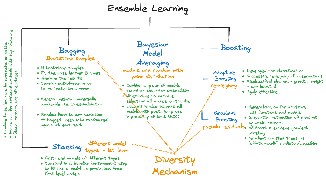
Figure 19.1 displays the main approaches in ensemble learning. What they all have in common is a mechanism by which diversity is introduced into the system and that diversity is exploited to gain strength.
Figure 19.1: An overview of approaches in ensemble learning
In stacking (also called stacked generalization), for example, base learners come from different model families. If the goal is classification of observations, base learners can be decision trees, logistic regression models, support vector machines, neural networks, naïve Bayes classifiers, and so on. Each of these has its strengths and weaknesses. The diversity of classification methods, once combined into a single classifier, hopefully combines the strengths of the methods and allays their weaknesses.
The base learners, whether homogeneous or heterogeneous, need to be combined into an overall output. In heterogeneous ensembles, another model, the so-called meta learner is built for that purpose. In homogeneous ensembles the combination is often a simple summing, averaging, or majority voting. This comes at the expense of interpretability—a single decision tree is intrinsically interpretable, a decision based on 500 trees built with different inputs and splits is much less interpretable. On the other hand, ensemble techniques can perform extremely well. So well that random forests or boosting methods such as gradient boosting machines or XGBoost have become de-facto standard approaches for many data scientists and machine learners.
To understand why ensembles are powerful, let’s take a look at a very simple situation: the sample mean in a random sample. Suppose we are drawing a random sample \(Y_1, \cdots, Y_n\) from a population with mean \(\mu\) and variance \(\sigma^2\). To estimate \(\mu\), we could use each of the \(Y_i\) as an estimator; after all, they are unbiased estimators for \(\mu\)\[
\text{E}[Y_i] = \mu, \quad \forall i
\]
The preferred estimator, however, is the sample mean \[
\overline{Y} = \frac{1}{n} \sum_{i=1}^n Y_i
\]
We prefer \(\overline{Y}\) over \(Y_i\) as an estimator of \(\mu\) because \[
\text{Var}[Y_i] = \sigma^2 \quad \text{Var}[\overline{Y}] = \frac{\sigma^2}{n}
\]
The variance of the sample mean can be made arbitrarily small by drawing a larger sample. The effect of reducing variability is particularly strong when \(\sigma^2\) is large. When \(\sigma^2 \rightarrow 0\), \(\overline{Y}\) provides less of an advantage as an estimator of \(\mu\) over \(Y_i\). And if \(\sigma^2 = 0\), then it makes no sense to draw more than a single observation: \(Y_1 = Y_2 = \cdots = Y_n = \mu\). After drawing one observation we know the mean.
Averaging has a very powerful effect on reducing variability. And that effect is stronger if the things being averaged are highly variable. Averaging things that do not vary does not buy as much. From these considerations flow two approaches to create a statistical model with small prediction error or high accuracy:
Carefully craft a single model that captures the variability in the data very well.
Average a bunch of models that have high variability and small bias.
You can see how the concept of diversity plays into homogeneous ensembles. The more variable–the more diverse–the base learners are, the more impact averaging has on their individual predictions or classifications.
19.2 The Bootstrap
The bootstrap is a powerful (re-)sampling procedure through which one can build up the empirical distribution of any quantity of interest. By taking a sufficiently large number of bootstrap samples, the empirical distribution can be made close to the real distribution of the quantity. Such a procedure has many applications, for example, to estimate the variability of a statistic or to average ensembles.
Suppose you have a data set of size \(n\). A bootstrap sample is a sample from the data, of the same size \(n\), drawn with replacement. The bootstrap procedure is to draw \(B\) bootstrap samples, repeat the analysis for each of them, and compute summary statistics (mean, standard deviation) across the \(B\) results.
Variance Estimation
Example: The Variance of \(R^2\)
One application of the bootstrap is to estimate the variability of a statistic. Take \(R^2\) in the classical linear model, for example. It is reported by software, but we never get an estimate of its standard error. Since \[
R^2 = 1 - \frac{\sum_{i=1}^n(Y_i - \widehat{Y}_i)^2}{\sum_{i=1}^n(Y_i - \overline{Y})}
\] depends on random variables, it is also a random variable. The bootstrap allows us to build up an empirical distribution of \(R^2\) values by resampling the data set over and over, fitting the linear model and computing its \(R^2\) each time, and then simply computing the standard deviation of the \(R^2\) values.
Suppose we wish to estimate the variance of \(R^2\) in a quadratic linear model predicting mileage per gallon from horsepower in the Auto data. The boot function in the boot library performs the bootstrap sampling based on a dataframe and a user-supplied function that returns the quantities of interest.
The array b$t contains the results computed from the \(B=1,000\) bootstrap samples. The \(R^2\) of the polynomial regression was 0.7067 in the first bootstrap sample, 0.6761 in the second bootstrap sample, and so on.
The \(R^2\) statistic for the original data is 0.6876. The std. error is the standard deviation of the 1000 bootstrap estimates of \(R^2\), sd(b$t) = 0.0283. The bias reported by boot is the difference between the mean of the bootstrap result and the estimate based on the original data:
mean(b$t) - b$t0
[1] 0.0007935389
How many bootstrap samples should you draw? The good news is that there is no overfitting when increasing \(B\). You need to draw as many samples as necessary to stabilize the estimate. Increase \(B\) to the point where the estimate does not change in significant digits.
sd(boot(data=Auto, boot.fn, R=2000)$t)
[1] 0.02869823
sd(boot(data=Auto, boot.fn, R=4000)$t)
[1] 0.02810885
sd(boot(data=Auto, boot.fn, R=5000)$t)
[1] 0.02795916
After several thousand bootstrap samples, the estimate of the standard deviation of \(R^2\) has stabilized to three decimal places. If we are satisfied with that level of accuracy, we have drawn enough bootstrap samples. If precision to four decimal places is required, \(B\) must be increased further.
Suppose we wish to estimate the variance of \(R^2\) in a quadratic linear model predicting mileage per gallon from horsepower in the Auto data. The boot_fn function in the following code returns the \(R^2\) for a second-order polynomial model in horsepower. np.random.choice draws the bootstrap samples with replacement.
import numpy as npimport pandas as pdfrom sklearn.preprocessing import PolynomialFeaturesfrom sklearn.linear_model import LinearRegressionfrom sklearn.metrics import r2_scoreimport seaborn as sns# Load the Auto dataset (equivalent to ISLR2::Auto)auto = sns.load_dataset('mpg').dropna()def boot_fn(data, index):"""Bootstrap function to compute R-squared for polynomial regression"""# Subset data using bootstrap indices X = data.iloc[index][['horsepower']] y = data.iloc[index]['mpg'] poly = PolynomialFeatures(degree=2, include_bias=False) X_poly = poly.fit_transform(X) reg = LinearRegression() reg.fit(X_poly, y)# Predict and calculate R-square y_pred = reg.predict(X_poly) r2 = r2_score(y, y_pred)return r2 # Bootstrap samplingnp.random.seed(123)n_samples =len(auto)B =1000# Perform bootstrapboot_results = []for i inrange(B):# Sample with replacement boot_indices = np.random.choice(n_samples, size=n_samples, replace=True) r2 = boot_fn(auto, boot_indices) boot_results.append(r2)boot_results = np.array(boot_results)print("First 10 bootstrap R-squared values:")
The array boot_results contains the results computed from the \(B=1,000\) bootstrap samples. The \(R^2\) of the polynomial regression was 0.6529 in the first bootstrap sample, 0.6718 in the second bootstrap sample, and so on.
# Original R-squaredoriginal_r2 = boot_fn(auto, np.arange(n_samples))def boot_sum(boot_results, original_r2):"""Function to summarize results of boot example"""print(f"\nOriginal R-squared: {original_r2:.6f}")print("\nBootstrap Statistics")print(f"Mean bootstrap R-squared: {np.mean(boot_results):.6f}")print(f"Bootstrap bias: {np.mean(boot_results) - original_r2:.6f}") print(f"Standard Deviation: {np.std(boot_results):.6f}\n")boot_sum(boot_results, original_r2)
Original R-squared: 0.687559

Bootstrap Statistics
Mean bootstrap R-squared: 0.688793
Bootstrap bias: 0.001234
Standard Deviation: 0.027915
The \(R^2\) statistic for the original data is 0.6876. The Standard Deviation is the standard deviation of the 1000 bootstrap estimates of \(R^2\), np.std(boot_results) = 0.0279. The bias is the difference between the mean of the bootstrap result and the estimate based on the original data.
How many bootstrap samples should you draw? The good news is that there is no overfitting when increasing \(B\). You need to draw as many samples as necessary to stabilize the estimate. Increase \(B\) to the point where the estimate does not change in significant digits.
# Standard errors for different bootstrap sample sizesdef get_bootstrap_se(n_boot):"""Get standard error for bootstrap with n_boot samples""" np.random.seed(123) # Reset seed for reproducibility results = []for i inrange(n_boot): boot_indices = np.random.choice(n_samples, size=n_samples, replace=True) r2 = boot_fn(auto, boot_indices) results.append(r2)return np.std(results)print(f"B=2000: {get_bootstrap_se(2000):.6f}")
B=2000: 0.028480
print(f"B=4000: {get_bootstrap_se(4000):.6f}")
B=4000: 0.028239
print(f"B=5000: {get_bootstrap_se(5000):.6f}")
B=5000: 0.028285
After several thousand bootstrap samples, the estimate of the standard deviation of \(R^2\) has stabilized to three decimal places. If we are satisfied with that level of accuracy, we have drawn enough bootstrap samples. If precision to four decimal places is required, \(B\) must be increased further.
Why are we introducing the bootstrap now, under ensemble learning? If the bootstrap procedure is useful to estimate a quantity, then we can use it to make predictions or classifications. The \(B\) bootstrap samples are variations of the original data, we can think of sampling with replacement as introducing diversity between the data sets and the resulting variability can be dampened by averaging. That is the idea behind bagging, a homogeneous ensemble method.
Out-of-bag Error
Before we move to bagging, it is insightful to learn more about the structure of the bootstrap samples. Since sampling is with replacement, some observations will appear once in the bootstrap sample, some will appear more than once, and others will not appear at all.
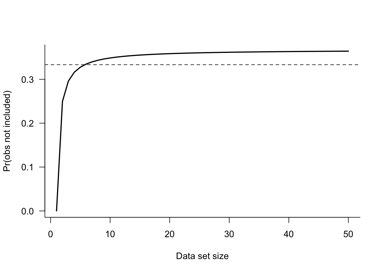
Consider a single bootstrap sample from a dataframe with \(n\) observations. The probability that the \(n\)th observation selected into the bootstrap sample is the \(j\)th observation in the data frame is \(1/n\), because sampling is with replacement. The complement, the probability that the \(n\)th bootstrap observation is not the \(j\)th obs is \(1-1/n\). It follows that in a bootstrap sample of size \(n\), the probability that a particular observation is not included is \[
(1 - 1/n)^n \approx 1/3
\]
As \(n\) grows, this probability quickly approaches 1/3. Figure 19.2 displays \((1-1/n)^n\) as a function of \(n\). The asymptote near 1/3 is reached for small data set sizes (> 10).
Figure 19.2: Probability that an observation is excluded from a bootstrap sample.
A bootstrap sample will contain about 2/3 of the observations from the original dataframe, some with repeated values. The other third of the observations are a natural hold-out sample for this bootstrap sample. The bootstrap procedure thus also provides a mechanism to estimate the test error similar to a cross-validation procedure. Two methods come to mind to use the bootstrap samples to estimate the test error:
In each of the \(B\) bootstrap samples, compute the test error based on the \(m\) observations not included in this sample. This set of observations is called the out-of-bag set
If the criterion is mean-squared prediction error, this would be for the \(j\)th bootstrap sample \[
\text{MSE}_{Te}^{(j)} = \frac{1}{m} \sum_{k=1}^m (y_k - \widehat{y}_k)^2
\] The overall test error is the average of the \(B\) out-of-bag errors: \[
\text{MSE}_{Te} = \frac{1}{B}\sum_{j=1}^B \text{MSE}_{Te}^{(j)}
\]
Another method of computing the out-of-bag error is to compute the predicted value for an observation whenever it is out-of-bag. This yields about \(B/3\) predicted values for each observation, and when averaged, an overall out-of-bag prediction for \(y_i\). The overall error is then computed from the \(n\) out-of-bag predictions. This estimate, for \(B\) sufficiently large, is equivalent to the leave-one-out prediction error, but it is not identical to the leave-one-out error because bootstrapping involves a random element and LOOCV is deterministic.
The following function computes the out-of-bag error estimates both ways for the Auto data and the model \[
\text{mpg} = \beta_0 + \beta_1\text{horsepower} + \beta_2\text{horsepower}^2 + \epsilon
\] and compares them to the LOOCV error:
Computing \(\text{MSE}_{Te}^{(j)}\) for each bootstrap sample and averaging those (a mean across \(B\) quantities)
Averaging the individual \(B/3\) out-of-bag predictions and computing the mean of those (a mean across \(n\) quantities)
Example: Out-of-bag Error Estimates Compared to LOOCV
OOB_error <-function(B=1000) { n <-dim(Auto)[1]# Compute LOOCV error first reg <-lm(mpg ~poly(horsepower,2), data=Auto) leverage <-hatvalues(reg) PRESS_res <- reg$residuals / (1-leverage) PRESS <-sum(PRESS_res^2) loocv_error <- PRESS/length(leverage); ind <-seq(1,n,1) MSE_Te <-0 oob_preds <-matrix(0,nrow=n,ncol=2)# draw the bootstrap samplesfor(i in1:B) { bs <-sample(n,n,replace=TRUE) # replace=TRUE is important here! oob_ind <-!(ind %in% bs) # the index of out-of-bag observations reg <-lm(mpg ~poly(horsepower,2), data=Auto[bs,])# predict the response for the out-of-bag observations oob_pred <-predict(reg,newdata=Auto[oob_ind,])# accumulate predictions of the out-of-bag observations oob_preds[oob_ind,1] <- oob_preds[oob_ind,1] + oob_pred oob_preds[oob_ind,2] <- oob_preds[oob_ind,2] +1# Accumulate mean-square prediction errors in the jth bootstrap sample MSE_Te <- MSE_Te +mean((oob_pred - Auto[oob_ind,"mpg"])^2) }# Average the MSE_Te^(j) across the B samples MSE_Te <- MSE_Te / B# Compute the average predictions for the n observations# oobs_preds[,2] will be approximately B/3 for each observation oob_preds[,1] <- oob_preds[,1] / oob_preds[,2] oob_error <-mean((oob_preds[,1]-Auto[,"mpg"])^2)return(list(MSE_Te=MSE_Te, OOB_error=oob_error, LOOCV=loocv_error))}set.seed(765)oe <-OOB_error(B=1000)oe