14 Classification with Random Inputs
14.1 Introduction
In Chapter 13 the approach to classification passed through a regression model. Characteristic of these models is that the mean of a random variable is modeled conditionally on the inputs. In other words, we assume that the \(X\)s are fixed. If they are random variables, then we condition the inference on the observed values. This is expressed simply in the conditional probabilities such as \[ \Pr(Y = j | \textbf{x}) \]
How would things change if we treat the \(X\)s as random variables?
Prior and Posteriors
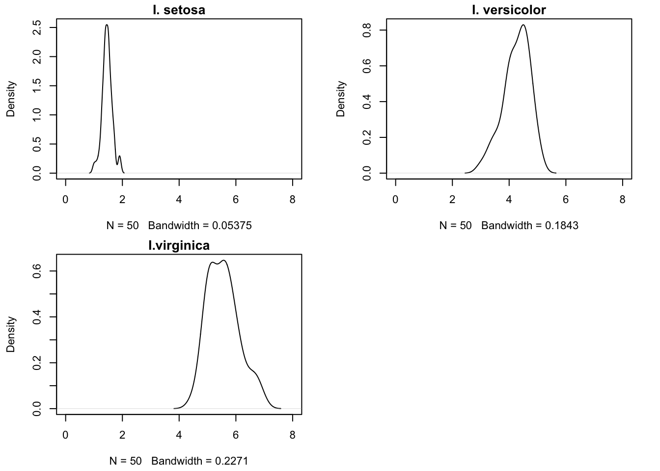
Recall the multinomial regression model in Section 13.2.1.2, modeling Iris species as a function of petal length. If we think of petal length as a random variable, we can study its distribution for each of the three species (Figure 14.1).
There is an overall probability that a randomly chosen Iris belongs to one of the species. Call this overall probability \(\pi_j = \Pr(Y=j)\). In a Bayesian context \(\pi_j\) is the prior probability to observe species \(j\). For each species \(j\), we now have a continuous distribution of the petal lengths:
- \(f_1(x)\) is the distribution of petal lengths for I. setosa
- \(f_2(x)\) is the distribution of petal lengths for I. versicolor
- \(f_3(x)\) is the distribution of petal lengths for I. virginica
Estimates of these densities are shown in Figure 14.1. These are conditional probabilities, \(\Pr(X | Y=j)\). Given those estimated densities and the prior probabilities of occurrence of the categories (species), can we classify an observation based on its input values? In other words, can we compute \(\Pr(Y=j | X=x)\) based on \(\pi_j = \Pr(Y=j)\) and \(\Pr(X | Y=j)\)?
Yes, we can, by applying Bayes’ Theorem: \[ \Pr(Y = j | X=x) = \frac{\pi_j f_j(x)}{\sum_{l=1}^k \pi_l f_l(x)} \tag{14.1}\]
Bayes Rule
The generic formulation of Bayes’ rule, for events \(A\) and \(B\) is \[ \Pr(A | B) = \frac{\Pr(A \cap B)}{\Pr(B)} = \frac{\Pr(A)\Pr(B|A)}{\Pr(B)} \] The rule allows us to reverse the conditioning from \(\Pr(B|A)\) to \(\Pr(A|B)\).
\(\pi_j\) is the prior probability that \(Y\) belongs to the \(j\)th class. In the absence of any additional information, if asked which Iris species you thinks a flower belongs to, you would go with the most frequent species. But now that we have seen data and can compute the distribution of petal lengths by species, we can use that information for a more precise calculation of the likelihood that \(Y\) belongs to category \(j\); \(\Pr(Y=j|X=x)\) is the posterior probability.
Applying this rationale to the Iris data, suppose we have not taken any petal length measurement. The species have the same estimate of the prior probability, \(\widehat{\pi}_j = 1/3\), because we have the same number of observations for each. If someone now tells you that they measured a petal length of 1.8, then given the densities in Figure 14.1, we should assign a high posterior probability that this is indeed a member of I. setosa. Similarly, for a petal length of 4.2, I. setosa is highly unlikely, I. versicolor is quite likely, but I. viriginica cannot be ruled out. If we have to settle on one category, we would side with the species that has the largest posterior probability.
The difference between the regression-based approach to classification and the methods in this chapter can be expressed as follows. In regression, we directly estimate \(\Pr(Y=j | \textbf{x})\). An alternative approach is to assemble this probability based on the prior probabilities \(\pi_j\) and the distribution of the inputs in the \(k\) categories.
Bayes Decision Boundary
Let’s consider the simple case where the \(X_j\) follow a \(G(\mu_j,\sigma^2)\) distribution. That means, they are Gaussian distributed and differ only in their means, not their variance. Plugging into Equation 14.1 with the normal density function for the \(f_j(x)\) yields \[ \Pr(Y = j | X=x) = \frac{\pi_j \frac{1}{2\pi\sigma}\exp\{-\frac{1}{2\sigma^2}(x-\mu_j)^2\}} {f(x)} \] In finding the category index \(j\) that maximizes the right hand side, the denominator can be ignored–it is the same for all categories. Maximizing the numerator is equivalent to maximizing its logarithm. This leads to the following classification rule: for a given value of \(x\), choose the category for which \[ \delta_j(x) = \text{ln}(\pi_j) + x\frac{\mu_j}{\sigma^2} - \frac{\mu_j^2}{2\sigma^2} \] is largest. The Bayes decision boundary between categories \(j\) and \(k\) is the value of \(x\) for which \(\delta_j(x) = \delta_k(x)\): \[ x = \frac{\sigma^2}{\mu_j - \mu_k} \left(\log(\pi_k) - \log(\pi_j) \right )+ \frac{\mu_j + \mu_k}{2} \]
If \(\pi_j = \pi_k\) this is simply \(x = (\mu_j + \mu_k)/2\), the average of the two means.
Figure 14.2 shows two Gaussian densities, \(G(-1,1)\) and \(G(1.5,1)\) and their 30:70 mixture. We can calculate the Bayes decision boundary with \(\mu_1 = -1\), \(\sigma^2 = 1\), \(\pi_1 = 0.3\), \(\mu_2 = 1.5\), and \(\pi_2 = 0.7\) as \[ x = \frac{1}{-1 - 1.5}(\log(0.7) - \log(0.3)) + \frac{-1+1.5}{2}=-0.08892 \]
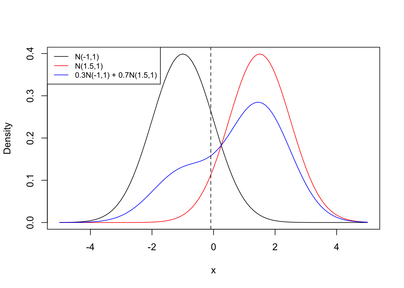
If you randomly draw an observation and its value is greater than \(x=-0.08892\) we conclude it comes from the \(G(1.5,1)\) distribution (category 2), if it is smaller we conclude it comes from the \(G(-1,1)\) distribution (category 1). If the value is exactly \(-0.08892\) then both distributions have equal posterior probabilities.
Simulation of Accuracy as Function of Decision Boundary
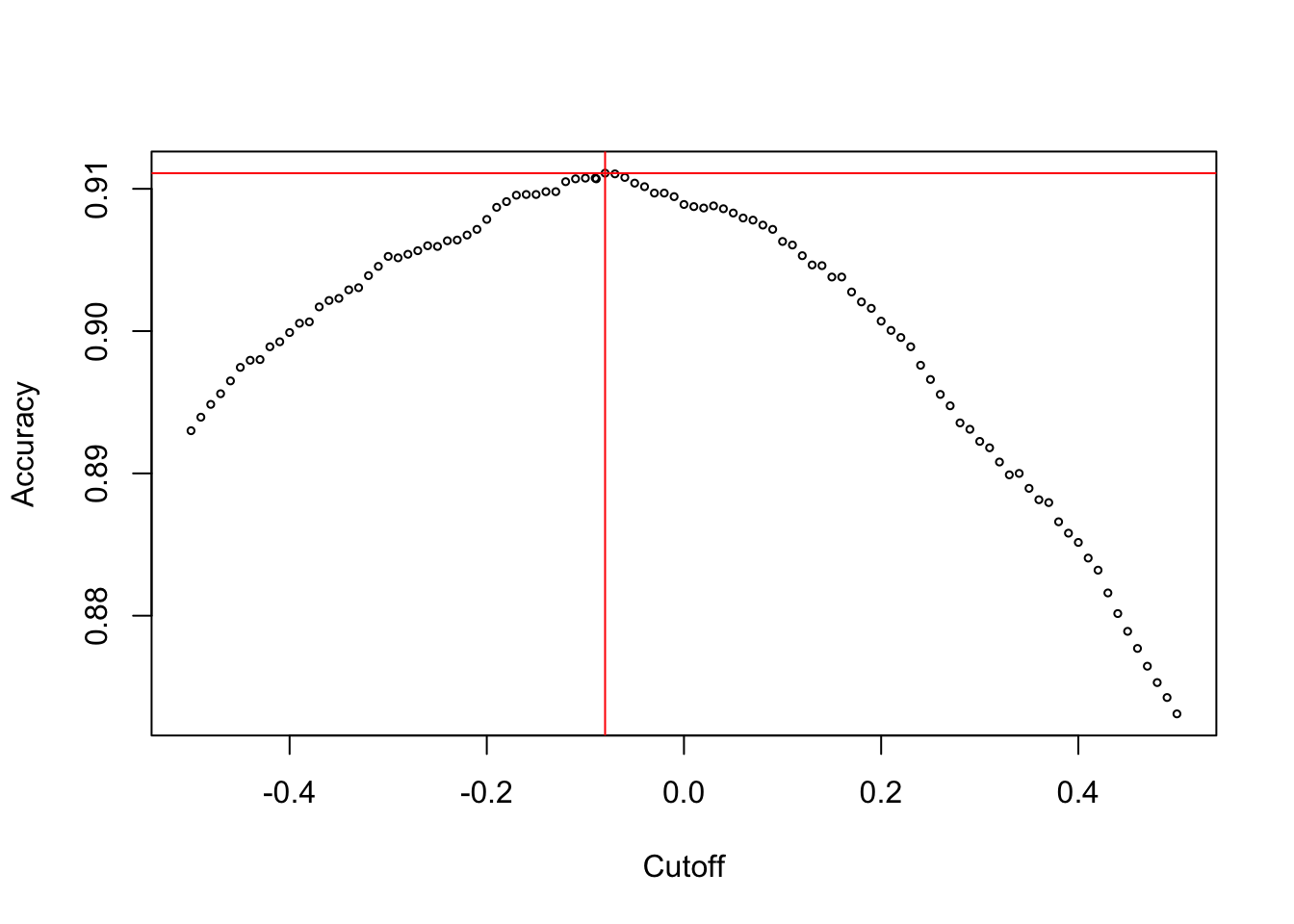
We can validate with a simulation that any other classifier that assigns observations to categories 1 and 2 based on a value other than \(x=-0.08892\) will have a larger misclassification rate (smaller accuracy).
We simulate 20,000 draws from Gaussian distributions with mean \(-1\) and \(1.5\) and variance \(1\). We also draw 20,000 times from a uniform(0,1) distribution which helps to create the mixture. If the uniform variable is less than 0.3 we choose an observation from the normal distribution with mean \(-1\), otherwise we choose from the distribution with mean \(1.5\). The decision boundary of \(x=-0.08892\) should have the greatest accuracy among all possible cutoffs if the experiment is repeated over and over.
set.seed(345)

x1 <- rnorm(20000,-1,1)
x2 <- rnorm(20000,1.5,1)
u <- runif(20000,0,1)

x1obs <- subset(x1, u < 0.3)
x2obs <- subset(x2, u >= 0.3)
data <- c(x1obs,x2obs)
Figure 14.3 shows the accuracy of the classifier as the cutoffs are varied. At the cutoff value \(-0.08992\) the highest accuracy is achieved (acc=0.908).
Two important methods that apply these ideas are discriminant analysis and the naïve Bayes classifier. They differ in assumptions about the distribution of the inputs.
14.2 Discriminant Analysis
Classification discriminant analysis (DA) was designed for the case of a qualitative target variable and one or more quantitative input variables. The typical assumption is that the input variables have a joint Gaussian distribution. When the distribution within each group is not known—or known not to be Gaussian—nonparametric forms of discriminant analysis that rely on kernel methods or nearest neighbor analysis are available.
At the heart of DA is the discriminant function, a decision rule used to classify observations into categories. The discriminant function is based on a generalized measure of distance between data points to the groups. This is a generalized distance because it takes into account the variances and covariances among the inputs. The posterior probabilities are functions of discriminant scores which are in turn based on those distances. An observation is assigned to the category which has the largest posterior probability.
Discriminant analysis is also a dimension reduction techniques, similar to principal component analysis (PCA, see Chapter 24). It computes one or more linear combinations between the quantitative variables that break down the variability between classes. In PCA, linear combinations are constructed that explain proportions of the total variability in the data.
Linear and Quadratic DA
Suppose we have \(p\) input variables \(X_1, \cdots, X_p\). Discriminant analysis assumes that the joint distribution of the inputs is multivariate Gaussian with mean vector \(\boldsymbol{\mu}= [\mu_1, \cdots, \mu_p]^\prime\) and covariance matrix \(\boldsymbol{\Sigma}\). A different multivariate Gaussian distribution applies to each of the \(k\) categories.
In linear discriminant analysis (LDA), the category-specific Gaussian distributions differ only in their mean vectors and not their covariance matrices. In quadratic discriminant analysis, the distributions differ in their mean vectors and their covariance matrices.
- LDA: \(f_j(\textbf{x}) \sim G(\boldsymbol{\mu}_j,\boldsymbol{\Sigma})\)
- QDA: \(f_j(\textbf{x}) \sim G(\boldsymbol{\mu}_j,\boldsymbol{\Sigma}_j)\)
We focus on LDA now.
Note that there are two “dimensions” to the problem. We have \(p\) inputs and \(k\) categories. For each of the \(j=1,\cdots,k\) categories we are dealing with a \(p\)-dimensional Gaussian distribution. With LDA, the p.m.f. for the \(j\)th distribution is
\[ f_j(\textbf{x}) = \frac{1}{(2\pi)^{p/2}|\boldsymbol{\Sigma}|^{1/2}} \exp\left\{ -\frac{1}{2} (\textbf{x}-\boldsymbol{\mu}_j)^\prime\boldsymbol{\Sigma}^{-1}(\textbf{x}-\boldsymbol{\mu}_j)\right \} \] where \(\boldsymbol{\mu}_j = [\mu_{j1},\cdots,\mu_{jp}]\). With \(p=3\), the covariance matrix \(\boldsymbol{\Sigma}\) has this form: \[ \boldsymbol{\Sigma}= \left [ \begin{array}{ccc} \ \text{Var}[X_1] & \text{Cov}[X_1,X_2] & \text{Cov}[X_1,X_3] \\ \text{Cov}[X_2,X_1] & \text{Var}[X_2] & \text{Cov}[X_2,X_3] \\ \text{Cov}[X_3,X_1] & \text{Cov}[X_3,X_2] & \text{Var}[X_3] \end{array} \right ] \]
The Bayes classifier assigns an observation with features \(\textbf{x}_0\) to the category \(j\) for which \[ \delta_j(\textbf{x}_0) = \textbf{x}_0^\prime\boldsymbol{\Sigma}^{-1}\boldsymbol{\mu}_j - \frac{1}{2}\boldsymbol{\mu}_j^\prime \boldsymbol{\Sigma}^{-1}\boldsymbol{\mu}_j + \text{ln}(\pi_j) \] is largest.
The term linear describes this form of discriminant analysis because \(\delta_j(\textbf{x}_0)\) is a linear function of the Xs—that is, the LDA decision rule depends on \(\textbf{x}\) only through a linear combination of its elements.
The assumption of a common variance across all categories helps to keep the number of parameters of the linear discriminant analysis in check. With \(k\) categories and \(p\) inputs the LDA has \(kp + p(p+1)/2\) parameters. This quickly escalates; with \(k=3\) and \(p=50\) we are dealing with 1,425 parameters.
In QDA the number of parameters is much larger because the covariance matrices are also category-specific. This leads to \(kp + kp(p+1)/2\) parameters. With \(k=3\) and \(p=50\) this results in 3,975 parameters.
Choosing between LDA and QDA is a classical bias-variance tradeoff. LDA is less flexible than QDA because of the equal-covariance-matrix constraint. If that constraint does not hold, LDA has high bias. QDA, on the other hand has high variability, in particular for small data sets where it is difficult to estimate variances and covariances well. If you have very large data sets or the common variance assumption is clearly wrong, choose QDA. Otherwise, give LDA a try.
Discriminant analysis has another glaring issue. The assumption of a joint multivariate Gaussian distribution of the inputs is questionable for many data sets. The assumption is a stretch for binary inputs such as those from encoding factors. Many continuous input variables are far from symmetric. The Gaussian assumption is for mathematical convenience, not because it reflects reality.
Discriminant Analysis in R
We can perform LDA with the MASS::lda function and QDA with the MASS:qda function in R.
Example: LDA for Iris Data
In Section 13.2.1.2, the Species variable of the Iris data was classified using a multinomial regression with one input, petal length. The model had an accuracy of 0.9583 on the test data set, only two I. versicolor were misclassified as I. virginica.
How does a linear discriminant analysis compare to the multinomial regression analysis?
First, we create the same train:test data split as in Section 13.2.1.2.
set.seed(654)
trainset <- caret::createDataPartition(iris$Species, p=2/3, list=FALSE,times=1)
iris_train <- iris[trainset,]
iris_test <- iris[-trainset,]

table(iris_train$Species)
    setosa versicolor  virginica
34 34 34 table(iris_test$Species)
    setosa versicolor  virginica
        16         16         16
The following statements compute the linear discriminant analysis and graph the results.
library(MASS)
iris_lda <- lda(Species ~ Petal.Length, data=iris_train)
iris_lda
Call:
lda(Species ~ Petal.Length, data = iris_train)
Prior probabilities of groups:
setosa versicolor virginica
0.3333333 0.3333333 0.3333333
Group means:
Petal.Length
setosa 1.461765
versicolor 4.247059
virginica 5.514706
Coefficients of linear discriminants:
LD1
Petal.Length 2.258558plot(iris_lda)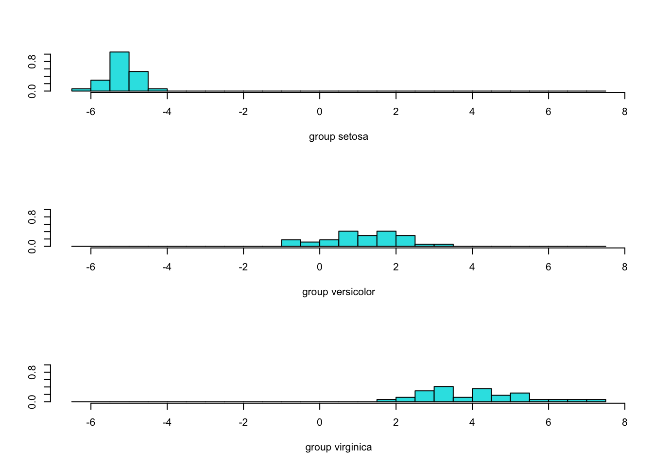
By default, lda uses the class proportions as the prior probabilities. Since each species has the same number of observations, the prior probabilities are the same. The next table in the output shows the average value of the input(s) in the classes. Only one discriminant function was computed, it explains all the between-class variability.
The graph shows the separation of the groups. With a single discriminant function, the graph consists of a series of histograms, one for each category. There is no overlap in the discriminant scores between I. setosa and the other species. I. versicolor and I. virginica show some overlap.
The confusion matrix tells us how well the LDA classifier does. It is identical to the confusion matrix in the multinomial regression model.
pred <- predict(iris_lda,newdata=iris_test)
caret::confusionMatrix(pred$class,iris_test$Species, mode="everything")
Confusion Matrix and Statistics
Reference
Prediction setosa versicolor virginica
setosa 16 0 0
versicolor 0 14 0
virginica 0 2 16
Overall Statistics
Accuracy : 0.9583
95% CI : (0.8575, 0.9949)
No Information Rate : 0.3333
P-Value [Acc > NIR] : < 2.2e-16
Kappa : 0.9375
Mcnemar's Test P-Value : NA
Statistics by Class:
Class: setosa Class: versicolor Class: virginica
Sensitivity 1.0000 0.8750 1.0000
Specificity 1.0000 1.0000 0.9375
Pos Pred Value 1.0000 1.0000 0.8889
Neg Pred Value 1.0000 0.9412 1.0000
Precision 1.0000 1.0000 0.8889
Recall 1.0000 0.8750 1.0000
F1 1.0000 0.9333 0.9412
Prevalence 0.3333 0.3333 0.3333
Detection Rate 0.3333 0.2917 0.3333
Detection Prevalence 0.3333 0.2917 0.3750
Balanced Accuracy 1.0000 0.9375 0.9688Next we return to the credit card default analysis from Section 13.1.
Example: Credit Default–ISLR (Cont’d)
Recall that the Default data is part of the ISLR2 library (James et al. 2021), a simulated data set with ten thousand observations. The target variable is default, whether a customer defaulted on their credit card debt. Input variables include a factor that indicates student status, account balance and income information.
As before, we randomly split the data into 9,000 training observations and 1,000 test observations.
library(ISLR2)
head(Default)
default student balance income
1 No No 729.5265 44361.625
2 No Yes 817.1804 12106.135
3 No No 1073.5492 31767.139
4 No No 529.2506 35704.494
5 No No 785.6559 38463.496
6 No Yes 919.5885 7491.559set.seed(765)
n <- nrow(Default)
testset <- sort(sample(n,n*0.1))
test <- Default[testset,]
train <- Default[-testset,]Linear discriminant analysis, LDA with equal priors, and quadratic discriminant analysis follow:
lda <- lda(default ~ income + balance + student, data=train)
lda
Call:
lda(default ~ income + balance + student, data = train)
Prior probabilities of groups:
No Yes
0.96688889 0.03311111
Group means:
income balance studentYes
No 33549.41 804.4596 0.2926913
Yes 32318.24 1749.8002 0.3859060
Coefficients of linear discriminants:
LD1
income 4.854450e-06
balance 2.248323e-03
studentYes -1.354917e-01lda2 <- lda(default ~ income + balance + student, data=train,
prior=c(0.5,0.5))
lda2Call:
lda(default ~ income + balance + student, data = train, prior = c(0.5,
0.5))
Prior probabilities of groups:
No Yes
0.5 0.5
Group means:
income balance studentYes
No 33549.41 804.4596 0.2926913
Yes 32318.24 1749.8002 0.3859060
Coefficients of linear discriminants:
LD1
income 4.854450e-06
balance 2.248323e-03
studentYes -1.354917e-01qda <- qda(default ~ income + balance + student, data=train)
qdaCall:
qda(default ~ income + balance + student, data = train)
Prior probabilities of groups:
No Yes
0.96688889 0.03311111
Group means:
income balance studentYes
No 33549.41 804.4596 0.2926913
Yes 32318.24 1749.8002 0.3859060Does the choice of linear versus quadratic DA and the choice of prior affect the classification performance?
lda_pred_test <- predict(lda, newdata=test)
lda_c <- caret::confusionMatrix(lda_pred_test$class,test$default,
                                positive="Yes")
lda_c$table
Reference
Prediction No Yes
No 961 29
Yes 4 6c(lda_c$overall[1],lda_c$byClass[1:2]) Accuracy Sensitivity Specificity
0.9670000 0.1714286 0.9958549 lda2_pred_test <- predict(lda2, newdata=test)
lda2_c <- caret::confusionMatrix(lda2_pred_test$class,test$default,
positive="Yes")
lda2_c$table Reference
Prediction No Yes
No 815 4
Yes 150 31c(lda2_c$overall[1],lda2_c$byClass[1:2]) Accuracy Sensitivity Specificity
0.8460000 0.8857143 0.8445596 qda_pred_test <- predict(qda, newdata=test)
qda_c <- caret::confusionMatrix(qda_pred_test$class,test$default,
positive="Yes")
qda_c$table Reference
Prediction No Yes
No 959 27
Yes 6 8c(qda_c$overall[1],qda_c$byClass[1:2]) Accuracy Sensitivity Specificity
0.9670000 0.2285714 0.9937824 The accuracy, sensitivity, and specificity of the default LDA and QDA are comparable, the QDA is slightly more sensitive, but neither model satisfies with respect to that metric.
Assuming equal priors, (lda2 analysis) means that prior to accounting for the inputs we assume that defaults and no defaults are equally likely. Under that (unreasonable) assumption the accuracy of the LDA classifier is lower but the sensitivity is much improved. A comparison of the classified values in the test set shows that 171 observations predicted as no defaults were classified as defaults under the equal prior assumption.
table(lda_pred_test$class, lda2_pred_test$class)
       No Yes
  No  819 171
  Yes   0  10
14.3 Naïve Bayes Classifier
Conditional Independence
The parametric discriminant analysis relies on a joint (multivariate) Gaussian distributions of the inputs. That does not accommodate qualitative (categorical) features. After converting those to 0–1 encoded binary columns, a Gaussian assumption is not reasonable. The naïve Bayes classifier (NBC) handles inputs of different types more gracefully—you can combine quantitative and qualitative inputs in the same classifier.
However, it does so by replacing the multivariate Gaussian assumption with another strong assumption: within a class \(j\) the \(f_j(\textbf{x})\) across the \(p\) inputs are independent (given the response \(Y\)).
Note
Note that \(f_j(\textbf{x})\) introduced earlier also has a conditional interpretation (\(f_j(\textbf{x}|y)\)). The conditioning on \(Y\) does not add anything new here.
The new wrinkle is that under the independence assumption the \(p\)-dimensional joint distribution of \([X_1,\cdots,X_p]\) for category \(j\) factors into the product of the marginal distributions \[ f_j(\textbf{x}|y) = f_{1}(x_1|Y=j) \times f_{2}(x_2 | Y=j) \times \cdots \times f_{p}(x_p | Y=j) \] Or, using our shorthand notation \[f_j(\textbf{x}|y) = f_{j1}(x_1) \times f_{j2}(x_2) \times \cdots \times f_{jp}(x_p) \]
Does this mean we are assuming \(X_1\) and \(X_2\) are independent? Not quite. It means that if you know that \(Y\) is in category \(j\), then knowing \(X_1\) has no bearing on our beliefs about \(X_2\). In other words, if we know that \(Y\) belongs to category \(j\), then \(f_j(x_2|y, x_1) = f_j(x_2|y)\): the distribution of \(X_2\) is not affected by the values of \(X_1\).
This is a very strong assumption. What did we gain by making it?
- Considerable simplification of the estimation procedure.
- We no longer have to model the \(p\)-dimensional joint distribution among the \(X\)s
- Features with different properties can be accommodated
- \(X_1\) might be continuous
- \(X_2\) can be a count
- \(X_3\) can be qualitative
- The distributions of the inputs can be estimated separately using different methods (kernel density, histogram, frequency distribution)
- The distributions do not have to be the same across categories. \(f_{j1}(x_1)\), the distribution of \(X_1\) in category \(j\) can be from a different distributional family than \(f_{k1}(x_1)\), the distribution of \(X_1\) in category \(k\).
The Classifier
The naïve Bayes classifier chooses as the predicted category of an observation the label for which \[ \Pr(Y= j | \textbf{x}) = \frac{\pi_j \times f_{j1}(x_1) \times \cdots \times f_{jp}(x_p)}{f(\textbf{x})} \] is largest. Since the denominator does not depend on \(Y\), this rule is equivalent to finding the category label for which \[ \pi_j \times f_{j1}(x_1) \times \cdots \times f_{jp}(x_p) \] is largest.
The prior probabilities \(\pi_l\) are estimated by the proportion of training observations in category \(j\). The densities \(f_{jm}(x_m)\) are estimated as follows:
- Quantitative \(X_m\):
- assume \(N(\mu_{jm},\sigma^2_{jm})\)
- or using a histogram of observations of the \(m\)th predictor in each class
- or using a kernel density estimator, essentially a smoothed histogram
- Qualitative \(X_m\):
- proportion of training observations for the \(m\)th predictor in each class
Naïve Bayes in R
Naive Bayes is implemented in R in various packages. The naiveBayes() function in the e1071 library uses syntax similar to that of lda and assumes that the numeric variables are Gaussian distributed. For factors (qualitative variables) it computes the conditional discrete distribution in each target category.
Example: Credit Default–ISLR (Cont’d)
library(e1071)
nb <- naiveBayes(default ~ income + balance + student, data=train)
nb
Naive Bayes Classifier for Discrete Predictors

Call:
naiveBayes.default(x = X, y = Y, laplace = laplace)

A-priori probabilities:
Y
        No        Yes
0.96688889 0.03311111

Conditional probabilities:
     income
Y         [,1]     [,2]
  No  33549.41 13323.37
  Yes 32318.24 13728.98

     balance
Y          [,1]     [,2]
  No   804.4596 454.9880
  Yes 1749.8002 344.5415

     student
Y            No       Yes
  No  0.7073087 0.2926913
  Yes 0.6140940 0.3859060
The information for the conditional probability distribution can be easily verified. For numeric variables (income, balance) the tables display the sample mean and sample standard deviation for each category. These are then used to calculate the \(f_j(x)\) as Gaussian densities.
library(dplyr)
# Prior probabilities
prior_freq <- table(train$default)
prior_freq/sum(prior_freq)
        No        Yes
0.96688889 0.03311111
# mean and standard deviation of income by default
train %>% group_by(default) %>%
summarize(income_mn=mean(income),
income_sd=sd(income))# A tibble: 2 × 3
default income_mn income_sd
<fct> <dbl> <dbl>
1 No 33549. 13323.
2 Yes 32318. 13729.# mean and standard deviation of balance by default
train %>% group_by(default) %>%
summarize(balance_mn=mean(balance),
balance_sd=sd(balance))# A tibble: 2 × 3
default balance_mn balance_sd
<fct> <dbl> <dbl>
1 No 804. 455.
2 Yes 1750. 345.# Proportions of students by default
t <- table(train$default,train$student)
t
        No  Yes
  No  6155 2547
Yes 183 115t[1,]/sum(t[1,]) No Yes
0.7073087 0.2926913 t[2,]/sum(t[2,]) No Yes
0.614094 0.385906 For example, the distribution of income given default=No is modeled as \[ f_{\text{No}}(\text{income}) = f(\text{income} | \text{default = No}) = G(33549.41,13323.37^2) \] and \[ f_{\text{Yes}}(\text{income}) = f(\text{income} | \text{default = Yes}) = G(32318.24,13728.98^2) \] The confusion matrix for the Naive Bayes estimates is identical to the confusion matrix of the logistic regression model:
nb_pred_test <- predict(nb,newdata=test)
nb_c <- caret::confusionMatrix(nb_pred_test,test$default, positive="Yes")
nb_c$table
Reference
Prediction No Yes
No 958 26
Yes 7 9c(nb_c$overall[1],nb_c$byClass[1:2]) Accuracy Sensitivity Specificity
0.9670000 0.2571429 0.9927461