33 Training Neural Networks
Training a neural network is in principle a nonlinear optimization problem: an objective function that is nonlinear in the parameters needs to be minimized (or maximized).
Note
We express all optimization problems as minimization problems. If you need to maximize a function \(\ell(\boldsymbol{\theta})\), you can always express it as a minimization problem with respect to \(-\ell(\boldsymbol{\theta})\). For example, maximum likelihood estimation (MLE) asks to find the values of \(\boldsymbol{\theta}\) that maximize the likelihood function, or, equivalently, the log likelihood function. Those are the values that minimize the negative log likelihood or minus twice the negative log likelihood. Finding MLEs by minimizing \(-2 \times \log \ell(\boldsymbol{\theta})\), where \(\ell\) is the likelihood function, is very common.
We will spend a few paragraphs on the general problem of finding the minimum of a function using iterative algorithms. While any of the general methods apply to ANNs in principle, neural networks present a set of specific challenges. The models are highly over-parameterized, the objective functions can be non-convex with multiple local minima and saddle points, the number of parameters is very large, the numerical precision in computing the all-important gradients can be questionable, etc. Because of these challenges specialized algorithms such as minibatch gradient descent with backpropagation have emerged to handle large neural networks specifically.
33.1 Nonlinear Function Optimization
Objective and Loss Functions
Suppose we have a function \(\ell(\boldsymbol{\theta};\textbf{y})\) of parameters and data and we wish to find estimates \(\widehat{\boldsymbol{\theta}}\) that minimize \(\ell(\boldsymbol{\theta};\textbf{y})\). We call \(\ell(\boldsymbol{\theta};\textbf{y})\) the objective function of the estimation problem. In many statistical learning and machine learning applications, \(\ell(\boldsymbol{\theta};\textbf{y})\) takes on the form of a sum over the observations, \[ \ell(\boldsymbol{\theta}; \textbf{y}) = \sum_{i=1}^n C_i(\boldsymbol{\theta};\textbf{y}) \] or an average, \[ \ell(\boldsymbol{\theta}; \textbf{y}) = \frac{1}{n} \sum_{i=1}^n C_i(\boldsymbol{\theta};\textbf{y}) \] where \(C_i\) is a measure of loss associated with observation \(i\).
In least-squares estimation, for example, \(C_i(\boldsymbol{\theta};\textbf{y})\) measures the squared error loss between the observed data and the model \(f(\textbf{x};\boldsymbol{\theta})\): \[ C_i(\boldsymbol{\theta};\textbf{y}) = \left(y_i - f(\textbf{x}_i;\boldsymbol{\theta}) \right)^2 \] In linear least squares, this loss simplifies to \[ C_i(\boldsymbol{\theta};\textbf{y}) = \left(y_i - \textbf{x}_i^\prime\boldsymbol{\theta}\right)^2 \] In maximum likelihood estimation, \(C_i(\boldsymbol{\theta}; \textbf{y})\) is the negative log likelihood function of the \(i\)th observation.
In statistical learning, loss functions are typically not divided by the number of observations. In machine learning (and in training neural networks) it is common to add the \(1/n\) divisor in the objective function. This is the difference between optimizing squared error loss or mean squared error loss, for example. It has no effect on the parameter estimates.
For training neural networks the most important loss functions when predicting a continuous target are
Squared error loss: \(C_i = (y_i - g(T(\textbf{a}^{(h)}))^2\).
Absolute error loss: \(C_i = |y_i - g(T(\textbf{a}^{(h)}))|\)
In classification models the most important loss functions are
binary cross-entropy loss (also called log-loss): \(C_i = - \left(y_i\log(\pi) + (1-y_i)\log(1-\pi)\right)\)
categorical cross-entropy loss: \(C_i = - \sum_{j=1}^k y_{ij} \log(\pi_j)\)
You will recognize the binary cross-entropy loss as the negative log likelihood of a Bernoulli(\(\pi\)) random variable and the categorical cross-entropy loss as the (kernel of) the negative log likelihood of a Multinomial(\(\pi_1,\cdots,\pi_k\)) random variable with \(k\) categories.
The Gradient
How do we go about finding the values of \(\boldsymbol{\theta}\) that minimize the objective function given a set of data? When the system has a closed-form solution, like the XOR problem in Section 32.2.4, we can compute the estimates in a single step. Most neural networks are not of that ilk and require an iterative, numeric solution: beginning from a set of starting values, the estimates are updated iteratively, with a general tendency toward improving (lowering) the objective function. When the objective function does not improve—or only negligibly so—the iterations stop.
In Section 9.3 we spent considerable energy on finding good starting values for nonlinear regression models. The closer the starting values are to a solution, the more reliably will any iterative algorithm improve on the starting values and converge. Recall the two-layer ANN for the MNIST data from the last chapter. The model has 109,386 parameters. How do you find starting values for all these? In the nonlinear regression models of Chapter 9 we relied on the intrinsic interpretability of the models to find starting values. Neural networks are not interpretable and any attempt to find “meaningful” starting values is futile. Usually, the starting values of neural networks are chosen at random.
Once we have starting values \(\boldsymbol{\theta}^{[0]}\), the objective function \(\ell(\boldsymbol{\theta}^{[0]};\textbf{y})\) can be computed.
Caution
The notation is a bit messy. We used superscripts with parentheses to identify layers in a neural network and now are using superscripts with square brackets to denote iterates of a parameter vector.
To improve on the starting values and get an updated value \(\boldsymbol{\theta}^{[1]}\), many optimization methods rely on the gradient of the objective function, the set of partial derivatives with respect to the parameter estimates. The gradient of the objective function is thus a vector, the size equals the number of parameters, and the typical element in position \(j\) is \[ \delta(\theta_j; \textbf{y}) = \frac{\partial \ell(\boldsymbol{\theta};\textbf{y})}{\partial \theta_j} \]
The overall gradient is the vector \(\boldsymbol{\delta}(\boldsymbol{\theta};\textbf{y}) = [\delta(\theta_1;\textbf{y}), \cdots, \delta(\theta_p;\textbf{y})]^\prime\).
The gradient measures the change in the objective function in the direction of \(\boldsymbol{\theta}_j\).
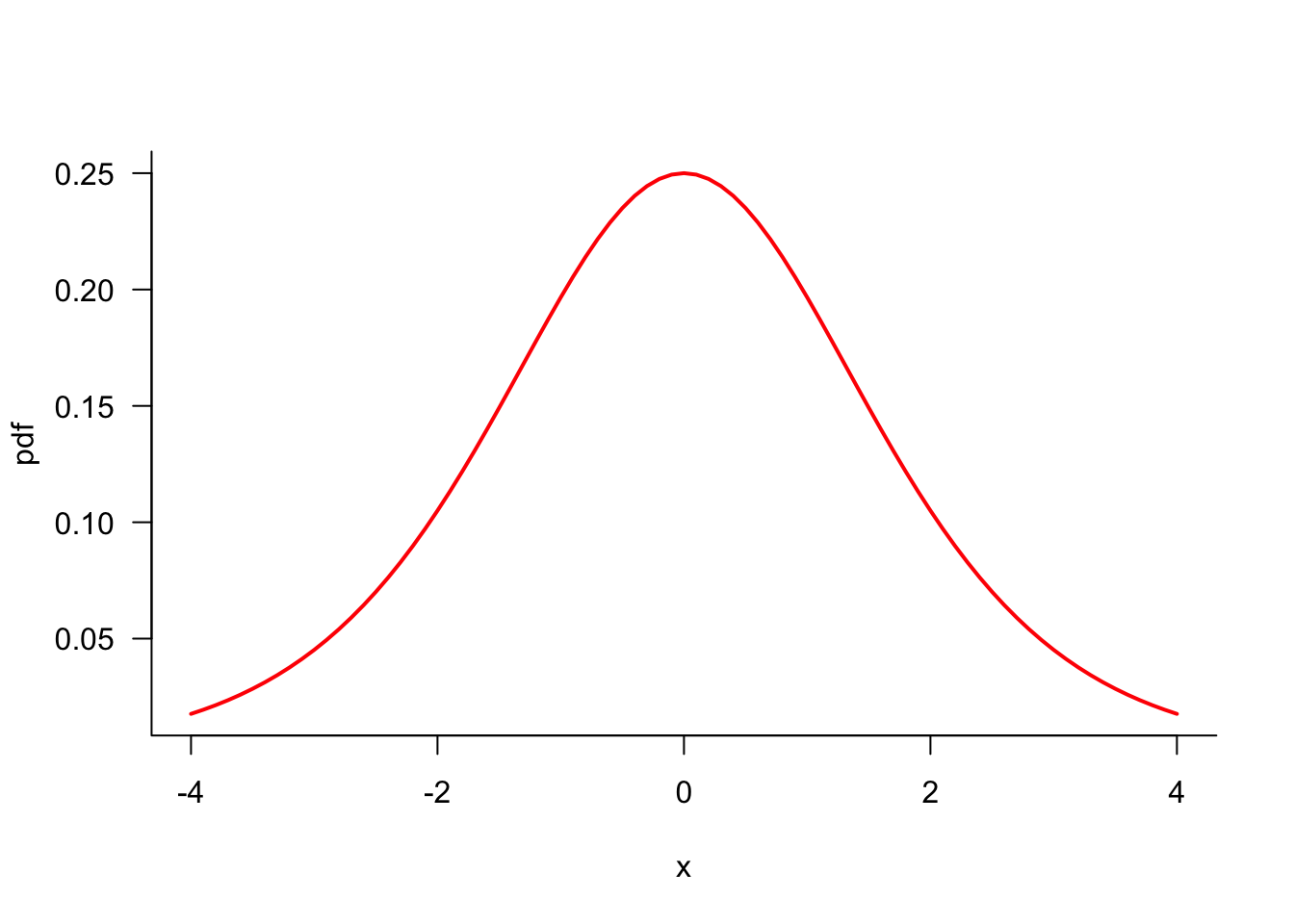
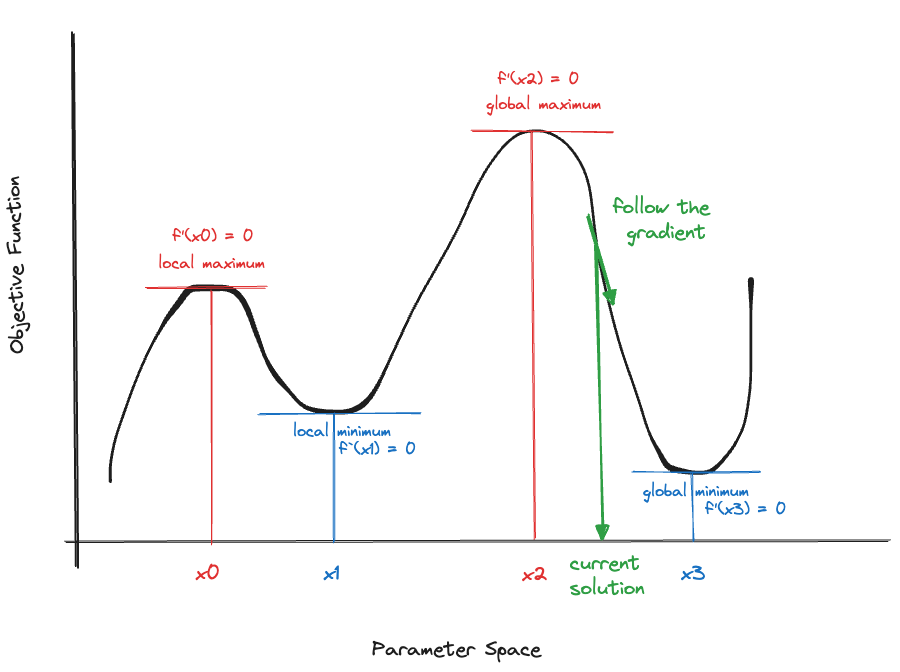
Using terminology and notation familiar from calculus, Figure 33.1 shows a function \(f(x)\) in one parameter (\(x\)). The function has two minima and two maxima. These occur at values of \(x\) where the derivative \(f^\prime(x)\) is zero. Once we have located a minimum or maximum, the second derivative \(f^{\prime\prime}(x)\) tells us whether we have found a minimum (\(f^{\prime\prime}(x) > 0\)) or a maximum (\(f^{\prime\prime}(x) < 0\)). Optimally we locate the overall minimum (or maximum), known as the global minimum (or maximum), not just a local minimum (maximum).
Suppose we started the search for a minimum at the value indicated with a green arrow in Figure 33.1. To find a smaller objective function value we should move to the right. Similarly, in Figure 33.2, we should move to the left.
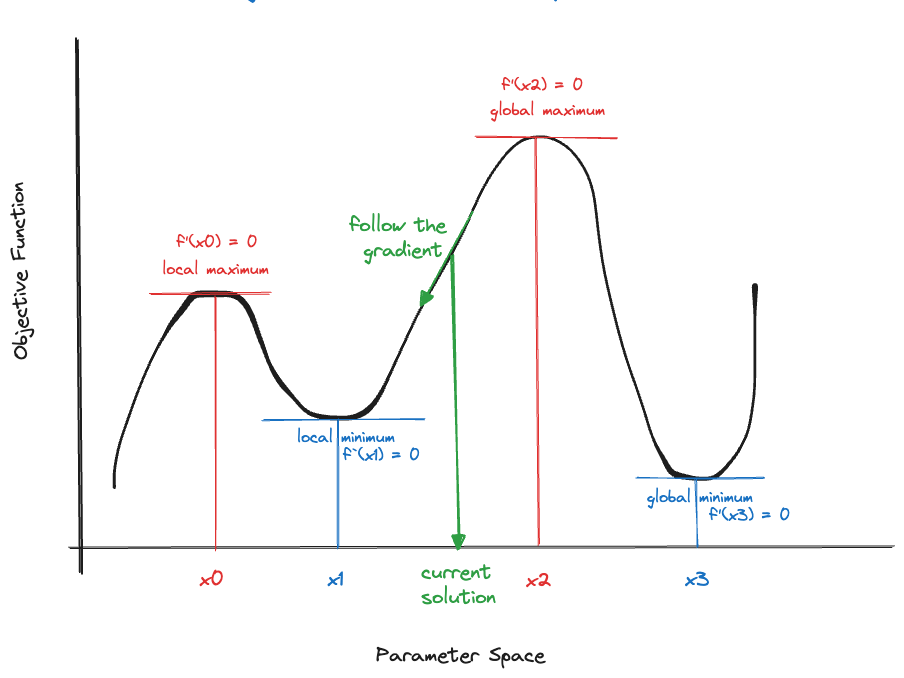
The upshot of the figures is that from any point in the parameter space, you should follow the negative value of the gradient to find a point in the parameter space where the objective function is lower. If we wanted to maximize the objective function, we would follow the direction of the positive gradient to climb up the objective function (Figure 33.3).
First-order methods
An optimization technique is called a first-order method if it relies only on gradient information to update the parameter estimates between iterations. The general expression for the update formula at iteration \(t\) is \[ \begin{align*} \boldsymbol{\delta}(\boldsymbol{\theta}^{[t]}; \textbf{y}) &= \frac{\partial{\ell(\boldsymbol{\theta};\textbf{y})}}{\boldsymbol{\theta}} \biggr\vert_{\boldsymbol{\theta}^{[t]}} \\ \boldsymbol{\theta}^{[t+1]} &= \boldsymbol{\theta}^{[t]} - \epsilon \times \boldsymbol{\delta}(\boldsymbol{\theta}^{[t]}; \textbf{y}) \end{align*} \tag{33.1}\]
\(\boldsymbol{\delta}(\boldsymbol{\theta}^{[t]}; \textbf{y})\) is the vector of derivatives of the objective function with respect to all parameters evaluated at \(\boldsymbol{\theta}^{[t]}\). The \((t+1)\)st value of the parameter estimates is obtained by moving \(\boldsymbol{\theta}^{[t]}\) in the direction of the negative gradient. The quantity \(\epsilon\) is known as the step size or the learning rate. It determines how big a step in the direction of the negative gradient we should take.
Examples of first-order optimization methods are
- Gradient descent
- Stochastic gradient descent
- Conjugate gradient algorithm
- Quasi-Newton algorithm
- Double dogleg algorithm
Note
The gradient tells us in which direction we need to apply a correction of the parameter estimates, it does not tell us how far we should go. Suppose you stand blindfolded in the vicinity of a cliff. You want to get closer to the cliff but not fall off it. Someone orients you toward the cliff. The learning rate determines the size of your next step. If you know that you are far away from the cliff you might as well take a full step—maybe even jump toward it. If you are very close to the cliff you only take a baby step.
The learning rate is an important hyperparameter of nonlinear optimization. Choosing a rate too small means making only tiny improvements and the procedure will require many iterations. Taking steps too large can make you miss a minimum and step from one valley of the objective function into another, giving the optimization fits. In nonlinear regression estimation, the best step size between iterations is often computed with a separate algorithm such as a line search. Machine learning applications range considerably in how they determine the learning rate. The classical stochastic gradient descent (SGD) algorithm holds \(\epsilon\) fixed throughout. The popular Adam optimizer, on the other hand, has a parameter-specific learning rate that is determined from the exponential moving average of the gradient and the squared gradient.
Second-order methods
Second-order optimization methods use information about the second derivative of the objective function in computing the updates. The second derivative contains information about the curvature of the objective function. The gradient tells us how much the objective function changes in a parameter, the curvature describes how much the function bends. Second-order information is captured by the Hessian matrix \(\textbf{H}\) of the objective function. The Hessian is simply the matrix of second derivatives of \(\ell(\boldsymbol{\theta};by)\) with respect to the parameters (the Jacobian of the gradient). The \((p \times p)\) Hessian matrix has typical element \[ \textbf{H}= [h_{ij}] = \frac{\partial^2{\ell(\boldsymbol{\theta};\textbf{y})}}{\partial \theta_i \partial \theta_j} \]
Examples of second-order optimization methods are the following:
- Fisher scoring
- Newton-Raphson algorithm
- Trust region algorithm
- Levenberg-Marquardt algorithm
Should you choose a first-order or second-order algorithm? All things being equal, second-order algorithms are superior to first-order algorithms and converge in fewer iterations. On the other hand, the computational effort for each iteration is much greater with a second-order algorithm. The parameter update between iterations is computed as \[ \boldsymbol{\theta}^{[t+1]} = \boldsymbol{\theta}^{[t]} - {\textbf{H}^{[t]}}^{-1}\boldsymbol{\delta}(\boldsymbol{\theta}^{[t]};\textbf{y}) \] and requires the computation and inversion of the \((p \times p)\) matrix \(\textbf{H}\). Recall the two layer ANN for the MNIST example from the last chapter. The model has 109,386 parameters. When \(p > 1000\), computing and inverting the Hessian at each iteration is prohibitive. Approximate methods such as limited memory BFGS (L-BFGS) exist. However, because of the generally large number of parameters, first-order methods dominate in training artificial neural networks; in particular variations of gradient descent.
33.2 Gradient Descent (GD) and Stochastic Gradient Descent (SGD)
The basic gradient descent algorithm was described above: to find the parameter values that minimize the objective function, take a step in the direction of the negative gradient: \[ \boldsymbol{\theta}^{[t+1]} = \boldsymbol{\theta}^{[t]} - \epsilon \times \boldsymbol{\delta}(\boldsymbol{\theta}^{[t]}; \textbf{y}) \]
The rationale is that the objective function decreases fastest in the direction of the opposite gradient. However, it is not guaranteed that \(\ell(\boldsymbol{\theta}^{[t+1]};\textbf{y}) \le \ell(\boldsymbol{\theta}^{[t]}; \textbf{y})\) if one takes a full step in the direction of the negative gradient. But the inequality should be true for some value \(\epsilon\), called the learning rate or step size.
An analogy to explain gradient descent is finding one’s way down from a mountain at night. You cannot see the path because of darkness, yet you need to descent from the mountain. The best way is to measure the slope in the vicinity of your location (compute the gradient), and to take a step in the direction of the greatest downhill slope. If you repeat this procedure you will either get off the mountain (find the global minimum) or get stuck in a depression (find a local minimum) such as a mountain lake.
In addition to changing the step length with the learning rate, we can also modify the direction in which we move downhill. The idea is that by taking a more shallow path the direction can be sustained for a longer period of time without measuring the slope again. This would reduce the number of gradient calculations, which can be expensive.
The classical gradient descent, also called batch GD, computes the gradient across all \(n\) observations in the training data set. When the objective function takes the form of a sum, \[ \ell(\boldsymbol{\theta}; \textbf{y}) = \frac{1}{n} \sum_{i=1}^n C_i(\boldsymbol{\theta};\textbf{y}) \] the gradient is the sum of the individual gradients \[ \delta(\theta_j; \textbf{y}) = \frac{\partial \ell(\boldsymbol{\theta};\textbf{y})}{\partial \theta_j} = \frac{1}{n} \sum_{i=1}^n \frac{\partial C_i(\boldsymbol{\theta};\textbf{y})}{\partial \theta_j} \] The parameters are updated after the gradients have been computed for all the parameters according to Equation 33.1. When \(n\) is large, computing the gradient can be time consuming. First-order methods tend to require more iterations until convergence and computing the gradient is a primary bottleneck of the algorithms.
The stochastic GD version is an online algorithm that computes gradients and updates one observation at a time: \[ \boldsymbol{\theta}^{[i+1]} = \boldsymbol{\theta}^{[i]} - \epsilon \boldsymbol{\delta}(\boldsymbol{\theta}^{[i]};y_i) \qquad i=1,\cdots,n-1 \] The true gradient is approximated as the gradient of the \(i\)th sample, and an update is calculated for each sample. This process of passing over the data and updating the parameters \(n\) times repeats until convergence, often with a random shuffling of the data between passes to avoid cycling of the algorithm.
Classical GD and SGD as presented here present the two extremes of calculating gradients between parameter updates: once for the entire sample, or for each observation. While the gradients computed in GD are very stable, they require the most computation between updates. The gradients in SGD on the other hand can be erratic and a poor approximation of the overall gradient. A compromise is minibatch gradient descent, where gradients are calculated for a small batch of observations, usually a few hundred.
SGD with minibatches and backpropagation has become a standard in training neural networks. The original SGD has a fixed learning rate, and an obvious extension is to modify the learning rate, for example, decreasing \(\epsilon\) with the iteration. The SGD algorithm then learns quickly early on and learns slower as the algorithm eaches convergence. Adaptive versions with a per-parameter learning rate are AdaGrad (Adaptive Gradient) and RMSProp (Root Mean Square Propagation). Since 2014, Adam-based optimizers (Adaptive Moment Estimation), an extension of RMSProp, have been used extensively in training neural networks due to their strong performance in practice.
Backpropagation
Working with neural networks you will hear and read about backpropagation. This is not a separate optimization algorithm, but an efficient method of calculating the gradients in a multi layer neural network. Because these networks are based on chaining transformations, you can express the gradient with respect to a parameter by the chain rule of calculus.
Backpropagation computes the gradient one layer at a time, going backward from the last layer to avoid duplicate computations, and using the chain rule.
33.3 Tuning a Network
-The performance of a neural network in training and scoring (inference) is affected by many choices. Training a neural network means tuning a sensitive and over-parameterized nonlinear problem; it is both art and science. Among the choices the model builder has to make are the following:
Hidden layers: number of layers, number of neurons in each layer, activation functions
Output function
Regularization parameters such as the dropout rate or the penalty for lasso or ridge regularization (see below)
Details of optimization: minibatch size, early stopping rule, starting values, number of epochs, learning rate, etc.
All of these should be considered hyperparameters of the network. With other statistical learning algorithms it is customary to determine values for some (or all) of the hyperparameters by estimation or by a form of cross-validation. With neural networks that is rarely the case. Training a single configuration of a network is time consuming and one often settles on a solution if the convergence behavior seems reasonable.
Regularization
Neural networks are over-parameterized. When we encountered high-dimensional problems previously in statistical learning, we turn to regularization and shrinkage estimation to limit the variability of the fitted function. That was the approach in ridge or lasso regression (Section 8.2) and in spline smoothing (Section 11.3.4).
Regularization in neural networks to reduce overfitting can take three different forms:
- \(L_1\) penalty (lasso-style) on a particular layer
- \(L_2\) penalty (ridge-style) on a particular layer
- Dropout regularization
Note that the regularization is applied on a per-layer basis, and not just as one big penalty term on the weights and biases of the entire network. Also, frameworks like TensorFlow or Keras allow you to add both regularization penalties separately for the weights, the biases, and/or the output of a layer. In Keras these are called the kernel_regularizer, bias_regularizer, and activity_regularizer, respectively. Each of those can apply an \(L_1\), an \(L_2\), or both penalties. As you can see, there are many choices and possible configurations. Typically, regularization penalties, whether \(L_1\) or \(L_2\) are applied to the weights of a layer, shrinking them toward zero. The bias terms, which act like intercepts are typically not regularized as that shrinks the model toward one that passes through the origin.
The new regularization method in the context of neural networks is dropout regularization, performed by adding a dropout layer to the network architecture. This is a parameter-free layer that randomly removes units from an input layer or a hidden layer by setting its activation to zero. Dropout learning can be applied to any layer, Figure 33.4 shows depicts a singe layer network with one input unit (\(x_3\)) and one hidden unit (\(A_2\)) being dropped.
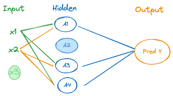
The dropped units do not receive connections from the preceding layer and do not emit output to the following layer.
Why does dropout learning work and reduce the chance of overfitting a neural network? Each neuron of a layer to which dropout is applied is removed with some probability \(\phi\). During training, the network cannot rely on any one neuron because it might disappear. As a result, assigning large weights to neurons is avoided in favor of spreading weights across the remaining nodes, making them smaller. As with \(L_1\) or \(L_2\) regularization, the effect of randomly dropping neurons from layers is to shrink the remaining weights to zero. Note that dropout can be applied to any layer and that the dropout rate \(\phi\) can vary among the dropout layers. Dropout rates range from \(\phi=0.1\) to \(\phi = 0.5\); yet another hyperparameter one has to think about.
While not regularizing a network can lead to overfitting, choosing a dropout rate or regularization penalty that is too high can lead to under-training the network that struggles to learn the patterns in the data.
Vanishing Gradients and Dying ReLU
Training neural networks with backpropagation computes the objective function on a forward pass through the network—from input layer to output layer—and the gradient on the backward pass—from output to input. The goal is to find values for weights and biases where the objective function has a minimum, a zero gradient. In nonlinear optimizations, the gradient thus naturally approaches zero as the iterations converge to a solution. When the gradient is near zero, the model “stops learning” and the process stops.
Vanishing gradients
The vanishing gradient problem describes the issue where the gradient values become very small and learning of the network slows down (or stops), simply because the gradients are small, not because we have found a minimum of the objective function. This affects deep networks more than shallow networks and the early layers suffer more from vanishing gradients than deep layers since the gradient is accumulated by moving backwards through the network.
The intuition for this phenomenon is that the overall gradient has a certain value, distributed across all the layers. As layers are chaining transformations, the overall derivative is essentially a long chain rule of products. If the values multiplied in this operation are small, the overall product can be tiny—the gradient is numerically vanishing.
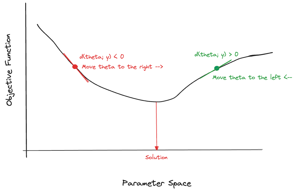
The vanishing gradient problem was more serious before the discovery of ReLU activation. The use of the sigmoid activation function contributed to vanishing gradients and limited the ability to train networks with many layers. To see why, consider the sigmoid activation \(\sigma(x) = 1/(1+\exp\{-x\})\) and its derivative. Since \(\sigma(x)\) is the c.d.f. of the standard logistic distribution, the derivative is the standard ogistic density function \[ f(x) = \frac{\partial \sigma(x)}{\partial x} = \frac{\exp^{-x}}{\left(1+\exp^{-x} \right)^2} \]
The density is symmetric about zero with a max value at zero of \(1/(1+1)^2 = 1/4\) (Figure 33.5). Because the gradient of the sigmoid activation function is \(\le 0.25\), repeated multiplication can produce very small numbers.
Dying ReLU
Why does ReLU help with the vanishing gradient problem? It partially helps because the function \(\sigma(x) = \max\{0,x\}\) has derivative \[ \frac{\partial \sigma(x)}{\partial x} = \left \{ \begin{array}{ll} x & x > 0 \\ 0 & x < 0 \end{array} \right . \] When \(x > 1\), multiplying with the gradient increases the product. However, for \(x \le 0\), the gradient is exactly zero and vanishes completely. The situation where many activations are negative, ReLU sets them to zero and essentially drops out the neuron, is known as the dying ReLU problem. Once the linear combinations \(b^{(t)}_j + \textbf{w}^{(t)}_j\textbf{a}^{(t-1)}\) are mostly in the negative range, the ReLU network cannot recover and dies. A large value for the learning rate will exacerbate this problem as it adjusts the parameter estimates downwards.
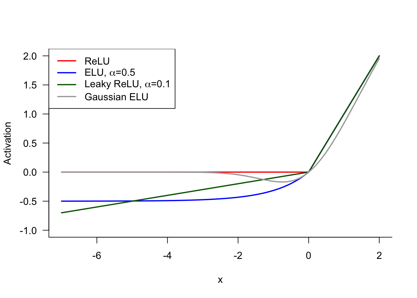
To address the dying ReLU problem and to help with the vanishing gradient issue, the leaky ReLU activation function has been proposed: \[ \sigma(x) = \left \{ \begin{array}{ll} x & x > 0 \\ \alpha x & x \le 0\end{array}\right . \] Leaky ReLU returns a small negative value when \(x < 0\), leading to a non-zero activation and a non-zero (albeit constant, \(\alpha\)) gradient. Values for \(\alpha\) in the range of 0.01 to 0.1 are common.
Related activation functions that avoid the dying ReLU issue are the *exponential linear unit (ELU) function \[ \sigma(x) = \left \{ \begin{array}{ll} x & x > 0 \\ \alpha (e^x-1) & x \le 0 \end{array}\right . \] and the Gaussian ELU** \[ \sigma(x) = x \,\Phi(x) \] where \(\Phi(x)\) is the standard Gaussian cumulative distribution function (Figure 33.6).
Another approach to minimize the odds of network training dying because of negative values, is to initialize the weights using positive values. Choosing random weights as starting points from a standard Gaussian or other distribution that is symmetric about zero, and a ReLU activation function, can cause many zero activations in early stages of training. Choosing random starting weights from distributions of positive random variables avoids this issue—we are assuming here that the inputs are positive-valued.
Scaling
Scaling the input variables is typically done for statistical learning methods that depend on measures of distance (clustering) or where the scale of inputs affects the distribution of variability (principal component analysis). In linear regression scaling the inputs by standardizing or normalizing is not really necessary unless he differences in scales across the inputs create numerical instability. Methods that regularize such as ridge or lasso regression often apply scaling internally to make sure that a common adjustment factor (the regularization penalty) applies equally to all coefficients.
Where do artificial neural networks fit in this? Should you consider scaling the input variables when training ANNs?
The answer is “Yes, usually you should” for the following reasons:
Neural networks are over-parameterized and very sensitive numerically. Numerical instabilities can throw them off and input variables with different scales is one source of instability that can be avoided.
The initial weights and biases are chosen at random, not taking into account the scale of the inputs. In order to get the optimization off well with random starting values, it is highly recommended that the inputs are on a similar scale.
The training epochs (iterations) are behaving no worse when the data are scaled. The optimization behavior is frequently better with scaled data.
One objection to scaling inputs in regression models is the changing interpretation of the coefficient. You need to know how the data were scaled in order to predict new values, for example. Neural networks are non-interpretable models, the actual values of the weights and biases is not of interest.
The recommended outcome of scaling inputs for neural networks is that all variables have a common range, and their values should be small, between 0 and 1. This suggests two approaches to scaling, standardizing and normalizing.
A variable is standardized by subtracting its mean and dividing by its standard deviation: \[ x_s = \frac{x-\overline{x}}{s_x} \] The resulting variable has arithmetic mean 0 and standard deviation 1.
A variable is normalized by shifting its range and scaling it to fall between 0 and 1: \[ x_n = \frac{x - \min\{x\}}{\max\{x\} - \min\{x\}} \]
Should you also scale the output variable? Some recommend it, but I do not. More important than scaling is making sure that the output activation function is chosen properly. For example, if the target variable \(Y\) is continuous and takes values \(-\infty < Y < \infty\), then you want an identity (“linear”) output function, and definitely not a ReLU function which would replace all negative values with 0. If, however, you choose a sigmoid or hyperbolic tangent output function, then scaling the output variable to range from 0–1 prior to training is necessary. To interpret the prediction from the neural network you would have to undo any scaling or normalization after the prediction.