In the previous chapter we analyzed longitudinal data with correlated error models. The example in Section 30.3.3 analyzed diameter measurements of 80 apples over a 12-week period. The fixed-effect model was a linear relationship between diameter and measurement time. If subscript \(i\) identifies the apple and subscript \(j\) the measurement occasion, the model for an individual observation is \[
Y_{ij} = \beta_0 + \beta_1 x_{ij} + \epsilon_{ij}, \quad i=1,\cdots,80
\] The graph of the fitted model with an autocorrelation structure of the \(\epsilon_{ij}\) is shown in Figure 30.9. All apples share the same intercept and slope. That seems problematic, some apples are clearly not represented well by that overall trend. In the vernacular of mixed models, this overall trend is called the population average trend for reasons that will become apparent soon.
How can we introduce more subject-specific behavior to capture that apples differ in their growth behavior? An obvious step would be to vary the intercepts and slopes between apples. The model \[
Y_{ij} = \beta_{0i} + \beta_{1i} x_{ij} + \epsilon_{ij}, \quad i=1,\cdots,80
\tag{31.1}\]
has a cluster-specific intercept and a cluster-specific intercept. These 80 intercepts and 80 slopes capture the variability in the fixed-effects among the clusters (apples).
Is there a more parsimonious way to express this variability? Replace in Equation 31.1\(\beta_{0i}\) with \(\beta_0 + b_0\) and \(\beta_{1i}\) with \(\beta_1 + b_1\): \[
Y_{ij} = (\beta_0 + b_{0i}) + (\beta_1 + b_{1i}) x_{ij} + \epsilon_{ij}, \quad i=1,\cdots,80
\tag{31.2}\]
The \(b_{0i}\) and \(b_{1i}\) terms in this model are random variables, not fixed effects. Specifically, we assume that \(b_{0i} \sim G(0,\sigma^2_0)\) and \(b_{1i} \sim G(0,\sigma^2_1)\). We are back to having only two fixed effects: \(\beta_0\) and \(\beta_1\). A specific apple’s intercept is expressed as a random deviation from the overall intercept. A specific apple’s slope is expressed as a random deviation from the overall slope.
Another way of thinking about the intercepts and slopes in Equation 31.2 is as follows: an effect consists of two elements: a fixed, overall, contribution and a random draw from a Gaussian distribution that is specific to the cluster (to the apple). Because the random effect is centered at 0, the overall contribution describes the behavior of the average apple. Adding the random draw yields the apple-specific effect. This explains the terms population-average and subject-specific effects. The behavior of the average apple is described by the population-average model \[
\text{E}[Y_{ij}] = \beta_0 + \beta_1 x_{ij}
\] The apple-specific behavior is described by the conditional model \[
\text{E}[Y_{ij} | b_{0i}, b_{1i}] = (\beta_0 + b_{0i}) + (\beta_1 + b_{1i}) x_{ij}
\]
What have we gained by introducing random effects \(b_{0i}\) and \(b_{1i}\) in Equation 31.2 compared to Equation 31.1?
A very natural way of expressing variability as normal random variation about a fixed value.
A more parsimonious way of expressing the variability in intercepts and slopes. Instead of 160 parameters in the mean function (80 \(\beta_{0i}\)s and 80 \(\beta_{1i}\)s) we have only four parameters: \(\beta_0, \beta_1, \text{Var}[b_{0i}] = \sigma^2_0, \text{Var}[b_{1i}] = \sigma^2_1\).
The ability to model the population average behavior and the cluster-specific behavior within the same model.
A straightforward way to address questions such as “do the slopes vary between clusters”? This is simply a test of \(H: \sigma^2_1 = 0\). If a random variable with mean 0 has variance 0, then it is the constant 0. If $= 0, then \(\beta_1 + b_{1i} = \beta_1\) and a common slope for all subjects is appropriate.
Definition
Definition: Mixed Model
A mixed model is a statistical model that contains multiple sources of random variation in addition to systematic (=fixed) effects. The random sources of variation separate into those describing the variability of model components and the variability of the target given all other effects.
Every major family of statistical model features a mixed model version. There are, for example, linear mixed models, nonlinear mixed models, generalized linear mixed models, generalized additive mixed models, and so on.
Counting the number of sources of random variation in the definition of a mixed model deserves some explanation. The issue arises because some models have a natural formulation in terms of additive errors. For example, the linear model for clustered data \[
\textbf{Y}_i = \textbf{X}_i\boldsymbol{\beta}+ \boldsymbol{\epsilon}_i
\] expresses the distributional properties of cluster target vector \(\textbf{Y}_i\) through the distributional properties of the model errors \(\boldsymbol{\epsilon}_i \sim (\textbf{0},\textbf{R}_i)\). This model contains one source of random variation, \(\boldsymbol{\epsilon}_i\). Adding a second random component, \(\textbf{Z}_i\textbf{b}_i\) where \(\textbf{b}_i \sim (\textbf{0},\textbf{D})\) is a random vector, creates a (linear) mixed model: \[
\textbf{Y}_i = \textbf{X}_i\boldsymbol{\beta}+ \textbf{Z}_i \textbf{b}_i + \boldsymbol{\epsilon}_i
\] This model now has two random sources of variation, \(\boldsymbol{\epsilon}_i\) and \(\textbf{b}_i\). The distribution of \(\textbf{Y}_i\) now can be interpreted in a population-average sense and in a cluster-specific sense: \[
\begin{align*}
\textbf{Y}_i &\sim (\textbf{X}_i\boldsymbol{\beta}, \textbf{Z}_i\textbf{D}\textbf{Z}_i^\prime + \textbf{R}_i) \\
\textbf{Y}_i | \textbf{b}_i &\sim (\textbf{X}_i\boldsymbol{\beta}+ \textbf{Z}_i\textbf{b}_i, \textbf{R}_i)
\end{align*}
\] —
In a generalized linear model the errors do not have an additive formulation. Instead, the distributional properties of the target are specified directly. For example, suppose that \(\textbf{Y}_i\) is a vector of (0,1) values that specify the disease state of an individual over time. For example, \(Y_{i1} = 1\) if subject \(i\) has the disease at the first observation occasion, and \(Y_{ij} = 0\) if the subject does not have the disease at the \(j\)th occasion. A generalized linear mixed model for this situation might specify \[
\begin{align*}
\textbf{Y}_i | \textbf{b}_i &\sim \text{Bernoulli}(\boldsymbol{\pi}_i) \\
\text{logit}(\pi_{ij} | \textbf{b}_i) &= \textbf{x}_{ij}^\prime \boldsymbol{\beta}+ \textbf{z}_{ij}^\prime\textbf{b}_i \\
\end{align*}
\] The expression for the linear predictor contains one random variable, \(\textbf{b}_i\). The second source of random variation is implied through assuming that \(\textbf{Y}_i\) conditional on the random effects, has a Bernoulli distribution.
Predicting Random Effects
Let’s return to the model with random intercept and random slopes in the apple example, Equation 31.2. The conditional (cluster-specific) and marginal (population-average) interpretations are elegant. With an estimate of \(\beta_0\) and \(\beta_1\), we can predict the population-average trend of apples as \[
\widehat{Y}_{ij} = \widehat{\beta}_0 + \widehat{\beta}_1 x_{ij}
\] How do we compute a cluster-specific prediction for the \(i\)th apple when \(b_{0i}\) and \(b_{1i}\) are unobservable random variables? We cannot estimate random variables, but fortunately, we can predict them. Based on the observed data and the distributional assumptions, values \(\tilde{b}_{0i}\) and \(\tilde{b}_{1i}\) can be found that are in some sense “best” guesses for the unobservable random variables. With those values the cluster-specific predictions can be computed: \[
(\widehat{Y}_{ij} | b_{0i}=\tilde{b}_{0i}, \,b_{1i}=\tilde{b}_{1i}) = \widehat{\beta}_0 + \tilde{b}_{0i} + (\widehat{\beta}_1 + \tilde{b}_{1i}) x_{ij}
\] Predictors of the random effects can be motivated in a number of ways, for example, by maximizing the joint density of \(\boldsymbol{\epsilon}\) and \(\textbf{b}\)(Henderson 1950, 1984) or by considering optimal unbiased predictors under squared-error loss (Harville 1976).
Prediction of Random Variables
We have encountered the issue of estimating parameters versus predicting random variables before. When predicting the target value for a new observation in regression models, we have a choice of estimating \(\text{E}[Y | x_0]\), the mean of the target at \(x_0\), or predicting \(Y | x_0\), the value of the random variable \(Y\) at \(x_0\). In discussing regression models, this is often presented as the difference between predicting the average at \(x_0\) or a single observation at \(x_0\).
In the classical linear model, the predicted values are the same for both, \(\widehat{y} = \textbf{x}_0\widehat{\boldsymbol{\beta}}\). What differs is the precision of that quantity. If we look for unbiased estimators that minimize squared error loss, then the relevant loss for predicting the mean is \(\text{Var}[\widehat{Y} - \text{E}[Y|x_0]]\) and for predicting \(Y|x_0\) it is \(\text{Var}[\widehat{Y}-Y]\). The former is the variance of \(\widehat{Y}\), the latter is the variance of a difference (since \(Y\) is a random variable)
So the good news is that by modeling the variation in the model terms through random effects, rather than through many fixed effects, we can calculate the solutions for the random effects and predict a cluster-specific response. This has an interesting implication for forecasting new values. We can forecast an apple’s diameter at any time point \(x_0\), even if it falls beyond the measurement period: \[
(\widehat{Y}_{ij} | b_{0i}=\tilde{b}_{0i}, \,b_{1i}=\tilde{b}_{1i}, x=x_0) = \widehat{\beta}_0 + \tilde{b}_{0i} + (\widehat{\beta}_1 + \tilde{b}_{1i}) x_0
\] How would we predict the response of a new apple, one that did not participate in the study? Our best estimates of the intercept and slope for this new apple are the population-average estimates \(\widehat{\beta}_0\) and \(\widehat{\beta}_1\). Unless we have reason to believe the new apple is not represented by the training data, we predict its diameter as \[
\widehat{Y}^* | x=x_0 = \widehat{\beta}_0 + \widehat{\beta}_1 x_0
\] What values for \(\tilde{b}_0\) and \(\tilde{b}_1\) are best for this new apple? If diameter measurements are available, and the apple did not contribute to the analysis, we can compute the predictors of the random effects. If diameter measurements are not available—the more realistic case—the random effects are best predicted with their mean, which is zero. In other words, the population-average prediction is the best we can do for new observations.
31.2 Linear Mixed Models
Note
Before “LMM” became the acronym for Large Language Model, it was the acronym for the Linear Mixed Model. LMM in this chapter refers to the linear mixed model.
Setup
Mixed models apply to many data structures. Longitudinal clustered data is a special situation where the data breaks into \(k\) clusters of size \(n_1, \cdots, n_k\). Split-plot experimental designs also have a linear mixed model representation, for example. To cover the more general case of the linear mixed model we do not explicitly call out the clusters with index \(i\). This makes the notation a bit cleaner. If you are thinking about a clustered data structure, where \(\textbf{Y}_i\) is the \((n_i \times 1)\) vector of responses for cluster \(i\), \(\textbf{X}_i\) is an associated matrix of inputs for the fixed effects, and \(\textbf{Z}_i\) is the matrix of inputs for the random effects, we now stack and re-arrange these as follows: \[
\textbf{Y}= \left [\begin{array}{c} \textbf{Y}_1 \\ \vdots \\ \textbf{Y}_k \end{array} \right]
\quad
\textbf{X}= \left [ \begin{array}{c} \textbf{X}_1 \\ \vdots \\ \textbf{X}_k \end{array}\right]
\quad
\textbf{b}= \left [\begin{array}{c} \textbf{b}_1 \\ \vdots \\ \textbf{b}_k \end{array} \right]
\quad
\boldsymbol{\epsilon}= \left [\begin{array}{c} \boldsymbol{\epsilon}_1 \\ \vdots \\ \boldsymbol{\epsilon}_k \end{array} \right]
\] The overall input matrix for the random effects is a block-diagonal matrix \[
\textbf{Z}= \left[
\begin{array}{cccc}
\textbf{Z}_1 & \textbf{0}& \cdots & \textbf{0}\\
\textbf{0}& \textbf{Z}_2 & \cdots & \textbf{0}\\
\vdots & \vdots & \ddots & \vdots \\
\textbf{0}& \textbf{0}& \cdots & \textbf{Z}_k
\end{array}
\right]
\] and the covariance matrices of the random effects and the model errors also take on a block-diagonal structure:
\[
\text{Var}[\textbf{b}] = \textbf{G}= \left[
\begin{array}{cccc}
\textbf{G}^* & \textbf{0}& \cdots & \textbf{0}\\
\textbf{0}& \textbf{G}^* & \cdots & \textbf{0}\\
\vdots & \vdots & \ddots & \vdots \\
\textbf{0}& \textbf{0}& \cdots & \textbf{G}^*
\end{array}
\right]
\qquad
\text{Var}[\textbf{b}] = \textbf{R}= \left[
\begin{array}{cccc}
\textbf{R}_1 & \textbf{0}& \cdots & \textbf{0}\\
\textbf{0}& \textbf{R}_2 & \cdots & \textbf{0}\\
\vdots & \vdots & \ddots & \vdots \\
\textbf{0}& \textbf{0}& \cdots & \textbf{R}_k
\end{array}
\right]
\] The variance matrix \(\text{Var}[\textbf{b}_i] = \textbf{G}^*\) is the same for all clusters. The variance matrix of the \(\boldsymbol{\epsilon}_i\) can differ from cluster to cluster, for example, when the observation times differ between clusters or in the presence of missing values.
With the re-arrangement from the clustered case out of the way, the general linear mixed model can be written as follows: \[
\begin{align*}
\textbf{Y}&= \textbf{X}\boldsymbol{\beta}+ \textbf{Z}\textbf{b}+ \boldsymbol{\epsilon}\\
\textbf{b}&\sim G(\textbf{0},\textbf{G}) \\
\boldsymbol{\epsilon}&\sim G(\textbf{0},\textbf{R}) \\
\text{Cov}[\textbf{b},\boldsymbol{\epsilon}] &= \textbf{0}
\end{align*}
\tag{31.3}\]
The assumption of Gaussian distributions for the random effects and the errors is common, it makes the subsequent analysis simple compared to any alternative specification. It should be noted that this implies a Gaussian distribution for \(\textbf{Y}\) as well. Applying the results for the multivariate Gaussian (Section 3.9), the conditional and marginal (population-average) distribution of \(\textbf{Y}\) is
The general linear mixed model Equation 31.3 contains parameters that need to be estimated and random variables that need to be predicted. The parameters are the fixed effects\(\boldsymbol{\beta}\) and the covariance parameters that define \(\textbf{G}\) and \(\textbf{R}\). In the longitudinal, clustered case, \(\textbf{R}\) has an autocovariance structure and \(\textbf{G}\) is often an unstructured matrix. For example, with a random intercept and a random slope, an unstructured \(\textbf{G}^*\) takes on the form \[
\textbf{G}^* = \left[\begin{array}{cc} \sigma^2_0 & \sigma_{01} \\ \sigma_{01} & \sigma^2_1 \end{array}\right]
\]\(\sigma^2_0\) and \(\sigma^2_1\) are the variances of the random intercept and slope, respectively, and \(\sigma_{01}\) is their covariance. Many other covariance structures are possbile for \(\textbf{G}\), including autocovariance structures when the random effects have a temporal or spatial structure.
We collect all covariance parameters into the vector \(\boldsymbol{\theta}= [\boldsymbol{\theta}_G, \boldsymbol{\theta}_R]\) and write the variance matrix of the data as a function of \(\boldsymbol{\theta}\): \[
\text{Var}[\textbf{Y}] = \textbf{V}(\boldsymbol{\theta}) = \textbf{Z}\textbf{G}(\boldsymbol{\theta}_G)\textbf{Z}^\prime + \textbf{R}(\boldsymbol{\theta}_R)
\]
Fixed effects and random effects
The mixed model equations are estimating equations for \(\boldsymbol{\beta}\) and \(\textbf{b}\) given that we know the covariance parameters \(\boldsymbol{\theta}\). These equations gp back to [Henderson (1950); Henderson1984] who derived them in the context of animal breeding. Henderson’s thought process was as follows: to derive estimating equations similar to the normal equations in least-squares estimation, consider the joint distribution of \([\boldsymbol{\epsilon}, \textbf{b}]\). We want to find the values \(\widehat{\boldsymbol{\beta}}\) and \(\widehat{\textbf{b}}\) which maximize this distribution.Since \(\boldsymbol{\epsilon}= \textbf{Y}- \textbf{X}\boldsymbol{\beta}- \textbf{Z}\textbf{b}\) and \(\textbf{b}\) are jointly Gaussian distributed and because \(\text{Cov}[\boldsymbol{\epsilon},\textbf{b}] = \textbf{0}\), maximizing their joint distribution for known \(\textbf{G}\) and \(\textbf{R}\) is equivalent to minimizing \[
Q = \textbf{b}^\prime\textbf{G}^{-1}\textbf{b}+ (\textbf{y}- \textbf{X}\boldsymbol{\beta}- \textbf{Z}\textbf{b})^\prime\textbf{R}^{-1}(\textbf{y}- \textbf{X}\boldsymbol{\beta}- \textbf{Z}\textbf{b})
\]\(Q\) is the sum of two quadratic forms, one in the random effects, the other in the model errors. Taking derivatives of \(Q\) with respect to \(\textbf{b}\) and \(\boldsymbol{\beta}\), setting to zero and rearranging yields the mixed model equations:
The solutions to Equation 31.4 are \[
\begin{align*}
\widehat{\boldsymbol{\beta}} &= \left(\textbf{X}^\prime\textbf{V}^{-1}\textbf{X}\right)^{-1}\textbf{X}^\prime\textbf{V}^{-1}\textbf{y}\\
\widehat{\textbf{b}} &= \textbf{G}\textbf{Z}^\prime\textbf{V}^{-1}(\textbf{y}- \textbf{X}\widehat{\boldsymbol{\beta}})
\end{align*}
\] The estimator of the fixed effects has the form of a generalized least squares estimator. The predictor of the random effects is a linear combination of the fitted residuals. Both results make sense. The random effects measure how much the conditional means differ from the marginal (population-average) prediction.
Note
Henderson’s method is not maximum likelihood although it was initially referred to as “joint likelihood estimation”. It is simply an intuitive way to motivate estimating equations for \(\boldsymbol{\beta}\) and \(\textbf{b}\). Harville (1976) established that the solution to the mixed model equations is a best linear unbiased predictor (BLUP) for \(\textbf{b}\) and remains the BLUP if the generalized least squares estimator for \(\boldsymbol{\beta}\) is substituted.
The mixed model equations Equation 31.4 are fascinating for another reason. Suppose we choose to estimate the inputs in \(\textbf{Z}\) not as random effects, but as fixed effects. That is, the model would be a linear model \[
\textbf{Y}= \textbf{X}\boldsymbol{\beta}_x + \textbf{Z}\boldsymbol{\beta}_z + \boldsymbol{\epsilon}, \qquad \boldsymbol{\epsilon}\sim (\textbf{0},\textbf{R})
\] The generalized least squares estimating equations for \(\boldsymbol{\beta}= [\boldsymbol{\beta}_x, \boldsymbol{\beta}_z]\) would be
\[
\left[\begin{array}{cc} \textbf{X}^\prime\textbf{R}^{-1}\textbf{X}& \textbf{X}^\prime\textbf{R}^{-1}\textbf{Z}\\
\textbf{Z}^\prime\textbf{R}^{-1}\textbf{X}& \textbf{Z}^\prime\textbf{R}^{-1}\textbf{Z}\end{array}\right]
\left[\begin{array}{c} \boldsymbol{\beta}_x \\ \boldsymbol{\beta}_z \end{array}\right] =
\left[\begin{array}{c} \textbf{X}^\prime\textbf{R}^{-1}\textbf{y}\\ \textbf{Z}^\prime\textbf{R}^{-1}\textbf{y}\end{array}\right]
\] These equations are very similar to the mixed model equations, except for the term \(+\textbf{G}^{-1}\) in the lower right cell of the first matrix. What does that mean? The inverse variance matrix \(\textbf{G}^{-1}\) acts like a shrinkage factor in the prediction of \(\textbf{b}\). If the variances of the random effects are small, the effect of \(\textbf{G}^{-1}\) on the estimating equations is large and the \(\textbf{b}\) will be shrunk toward zero compared to the fixed-effect estimates. On the contrary, when the variances of the random effects are large, there will be less shrinkage in the random effects solution.
Covariance parameters
Covariance parameters can be derived by a number of principles, once the parameter estimates are obtained you plug them into \(\textbf{G}\) and \(\textbf{R}\) and solve the mixed model equations. The most important estimation principles for the estimation of covariance parameters are maximum likelihood (ML) and restricted (residual) maximum likelihood (REML) based on the marginal distribution of \(\textbf{Y}\), as for the general correlated error model discussed in Section 30.3.
Since \(\textbf{Y}\) is multivariate Gaussian, minus twice the negative log likelihood is \[
-2 \ell(\boldsymbol{\theta},\boldsymbol{\beta};\textbf{y}) = \log |\textbf{V}(\boldsymbol{\theta})| + (\textbf{y}-\textbf{X}\boldsymbol{\beta})^\prime\textbf{V}(\boldsymbol{\theta})^{-1}(\textbf{y}-\textbf{X}\boldsymbol{\beta}) + c
\tag{31.5}\] where \(c\) is a constant that does not depend on the parameters. Given \(\boldsymbol{\theta}\), the minimum of \(-2 \ell(\boldsymbol{\theta},\boldsymbol{\beta};\textbf{y})\) with respect to \(\boldsymbol{\beta}\) has a closed-form solution in the GLS estimator \(\widehat{\boldsymbol{\beta}} = (\textbf{X}^\prime\textbf{V}^{-1}\textbf{X})^{-1}\textbf{X}^\prime\textbf{V}^{-1}\textbf{y}\). Plugging this estimator back into Equation 31.5 leads to a function in \(\boldsymbol{\theta}\) only. The ML estimates of \(\boldsymbol{\theta}\) are found by numerically minimizing this profiled log-likelihood.
In the case of REML, instead of the log-likelihood of \(\textbf{Y}\) one maximizes the log-likelihood of \(\textbf{K}\textbf{Y}\) where \(\textbf{K}\) is a matrix of error contrasts chosen such that \(\textbf{K}\textbf{X}= \textbf{0}\). A common choice of \(\textbf{K}\) leads to the following expression for minus twice the restricted log-likelihood \[
-2 \ell(\boldsymbol{\theta};\textbf{y}) = \log |\textbf{V}(\boldsymbol{\theta})| + \log |\textbf{X}^\prime\textbf{V}(\boldsymbol{\theta})^{-1}\textbf{X}| + (\textbf{y}-\textbf{X}\boldsymbol{\beta})^\prime\textbf{V}(\boldsymbol{\theta})^{-1}(\textbf{y}-\textbf{X}\boldsymbol{\beta}) + c_R
\tag{31.6}\]
This is the same objective function as Equation 31.5 except for the second log determinant term (and the inconsequential constant terms). Also notice that the REML log-likelihood is a function of only the covariance parameters. The fixed effects are not profiled from Equation 31.6. The fixed effects are removed by considering the special transformation \(\textbf{K}\textbf{Y}\).
REML estimators of the covariance parameters are generally less biased than ML estimates, and are sometimes unbiased. They are preferred for this reason. However, the restricted log-likelihood in Equation 31.6 does not contain information about the fixed effects. You cannot use the restricted log-likelihood to perform likelihood ratio tests for hypotheses about the fixed effects.
Choosing Random Effects
When a mixed model arises in the context of an experimental design—such as a split-plot design—the assignment of fixed and random effects is dictated by the experimental design. In other situations, there is more latitude in choosing fixed and random effects.
Example: Sleep Study.
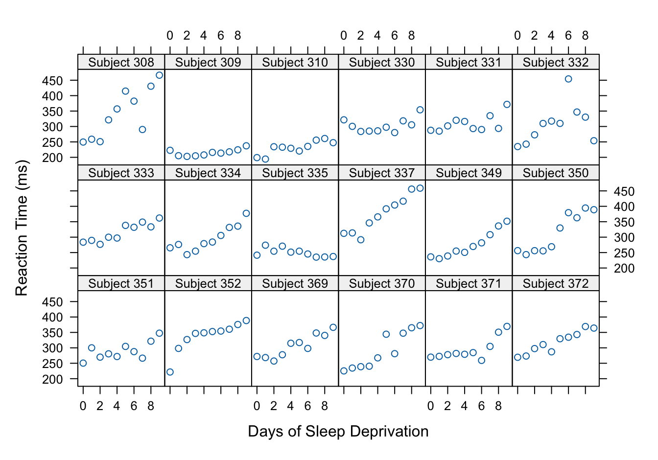
The data for this example are part of the lme4 library in R and represent the average reaction time (in milliseconds) for subjects in a sleep deprivation study. The data are a subset of a larger study described in Belenky et al. (2003).
Figure 31.1 shows the response profiles for the 18 subjects in the study. In general, the reaction times increase with increasing sleep deprivation. However, there is clearly substantial subject-to-subject variability in the profiles. Some subjects (#309, #310) do not respond to sleep deprivation very much compared to others (#308, #337, for example). The trend of reaction time versus duration of sleep deprivation could be linear for most subjects, quadratic for some.
If we assume a linear trend for all subjects, do the intercepts and slopes vary across subjects or only the intercepts or only the slopes?
library(lme4)library(lattice)xyplot(Reaction ~ Days | Subject, data=sleepstudy,xlab="Days of Sleep Deprivation",ylab="Reaction Time (ms)",strip =function(...) {strip.default(..., strip.names =TRUE, strip.levels=TRUE,sep=" ") },par.strip.text =list(cex =0.8), type=c("p"),layout=c(6,3,1),as.table=TRUE )
Figure 31.1: Reaction times by subject in sleep deprivation study
As a general rule, if a coefficient of a linear model appears in the random part of the model it should be included in the fixed effects part. Otherwise it might not be reasonable to assume that the random effects have a zero mean. In the sleep deprivation study, this means a model such as \[
Y_{ij} = \beta_0 + b_{1i} x_{ij} + \epsilon_{ij}
\] with a random slope but no fixed-effect slope is not appropriate. In order for the \(b_{1i}\) to satisfy a zero-mean assumption, there needs an overall (population-average) slope in the model:
\[
Y_{ij} = \beta_0 + \beta_1 x_{ij} + b_{1i} x_{ij} + \epsilon_{ij}
\] In other words, the columns in \(\textbf{Z}\) also appear in \(\textbf{X}\). The reverse is not necessarily so. Not varying the intercepts or slopes by subject is perfectly acceptable.
Linear Mixed Models in R
Linear mixed models cam be fit in R with the lme4 and nlme packages. nlme fits LMMs with the lme function and nonlinear mixed models with the nlme() function by ML or REML. lme4 fits LMMs with the lmer() function by ML or REML, generalized linear models with the glmer() function by ML, and nonlinear mixed models with the nlmer() function by ML.
Example: Sleep Study (Cont’d)
We use lme for the analysis of the sleep study data because it allows us to specify random effects and a correlated within-subject error structure. The model we have in mind is \[
\begin{align*}
Y_{ij} &= \beta_0 + \beta_1 d_{j} + b_{0i} + b_{1i}d_j + \epsilon_{ij} \\
\textbf{G}^* &= \left [\begin{array}{cc}\sigma^2_0 & \sigma_{01} \\ \sigma_{01} & \sigma^2_1 \end{array}\right] \\
\text{Cov}[\epsilon_{ij},\epsilon_{ik}] &= \sigma^2 \rho^{|d_j - d_k|}
\end{align*}
\] where \(Y_{ij}\) is the sleep deprivation of subject \(i\) on day \(d_j\) (\(i=1,\cdots,18\)). This is a linear mixed model with random intercept and slopes and correlated errors. The autocovariance structure is that of a continuous AR(1) process. There are a total of seven parameters in this model:
the population-average intercept \(\beta_0\) and the population-average slope \(\beta_1\)
the variances of the random effects, \(\sigma^2_0\) and \(\sigma^2_1\) and their covariance \(\sigma_{01}\)
rhe variance of the errors, \(\sigma^2\)
the autocorrelation \(\phi\)
The following statements fit this model by REML (the default) using lme.
The fixed= argument specifies the fixed effects of the model, an intercept is included automatically. The random= argument specifies the random effects and the clusters after a vertical slash. The intercept is not automatically included in the random effect specification. The covariance structure is specified with the correlation= argument using the same syntax as the correlated error model in Section 30.3.3. The control= argument changes the numerical optimizer from the default to a general purpose algorithm.
Linear mixed-effects model fit by REML
  Data: sleepstudy
       AIC     BIC    logLik
  1738.187 1760.46 -862.0935

Random effects:
 Formula: ~1 + Days | Subject
 Structure: General positive-definite, Log-Cholesky parametrization
            StdDev    Corr
(Intercept) 14.879196 (Intr)
Days         4.759861 0.897
Residual    30.500694

Correlation Structure: AR(1)
 Formula: ~Days | Subject
 Parameter estimate(s):
      Phi
0.4870368
Fixed effects:  Reaction ~ Days
                Value Std.Error  DF  t-value p-value
(Intercept) 252.24315  6.851137 161 36.81770       0
Days         10.46701  1.532133 161  6.83166       0
 Correlation:
     (Intr)
Days -0.131

Standardized Within-Group Residuals:
        Min          Q1         Med          Q3         Max
-3.18606983 -0.63340364  0.06086905  0.49755434  4.78980880

Number of Observations: 180
Number of Groups: 18
The estimates of the fixed effects are \(\widehat{\beta}_0\) = 252.2432 and \(\widehat{\beta}_1\) = 10.467.
The estimates of the covariance parameters are \(\widehat{\sigma}^2_0\) = 221.3905, \(\widehat{\sigma}^2_1\) = 22.6563, and \(\widehat{\sigma}_{01}\) = 63.509. The lme output reports the square roots of the variances (Std Dev) and reports the correlation between \(b_{0i}\) and \(b_{1i}\) rather than the covariance.
The estimate of the autocorrelation parameter is \(\widehat{\phi}\) = 0.487.
The model with random effects and autocorrelated errors has a restricted log-likelihood of -862.0935. We can test if the addition of the correlation process significantly improves the model by comparing this model against one without the correlation structure. If we fit both models by REML, this is a valid likelihood ratio test of \(H: \phi = 0\).
         Model df      AIC      BIC    logLik   Test  L.Ratio p-value
lmix         1  6 1755.628 1774.719 -871.8141
lmixcorr     2  7 1738.187 1760.459 -862.0935 1 vs 2 19.44123  <.0001
The model without correlated errors has a restricted log likelihood of -871.8141. Twice the difference of the log-likelihoods is the test statistic for the LRT, 19.4412. There is one restriction on the full model, \(\phi=0\), hence this is a 1-degree of freedom test. The \(p\)-value is very small, we reject the hypothesis that \(\phi = 0\). The correlated error structure is significant, we continue our investigation with the lmixcorr model.
The fixed and random effects can be extracted with the respective access functions:
The random effects are organized as a matrix, the columns correspond to the intercept and slope, the rows correspond to subjects. To predict the response for the average study participant, we use intercept and slope estimates \(\widehat{\beta}_0\) = 252.2432 and \(\widehat{\beta}_1\) = 10.467.
To predict the sleep deprivation of subject #333, we use the subject-specific intercept and slope \(\widehat{\beta}_0 + b_{0,333}\) = 252.2432 + 5.1421 = 257.3853, \(\widehat{\beta}_1 + b_{1,333}\) = 10.467 + 1.3911 = 253.6343.
With increasing time of sleep deprivation, which subject has the smallest increase in reaction time and which subject has the largest increase?
To answer this question we can look at the min and max of the random slope predictors:
Subjects 330, 334, 370, and 371 are similar to the population average. They have the smallest subject-specific intercept and slope adjustment.
This is also confirmed in Figure 31.2 below. The subject-specific and population-average predictions for these four subjects overlay closely.
What is the predicted reaction time on day 4 for an individual who did not participate in the study?
To answer this question we have to rely on the population average effects since we do not have a solution for the random effects predictor.
pred <-fixed.effects(lmixcorr)[1] +4*fixed.effects(lmixcorr)[2]cat ("Predicted reaction time of a new subject at day 4 = ", pred)
Predicted reaction time of a new subject at day 4 = 294.1112
You can also use the predict() function but when you do that for a subject that is not in the study you get a NA. To get around that and obtain the population-average predictions, specify the level= option of predict(). Check the doc on predict.lme() for details. If you specify level=0 it does not matter what you pass for the Subject variable. You can even leave it out of the data frame.
# Subject in the study, population-average predictionsdata <-data.frame("Days"=4,"Subject"=308)predict(lmixcorr,newdata=data,level=0)
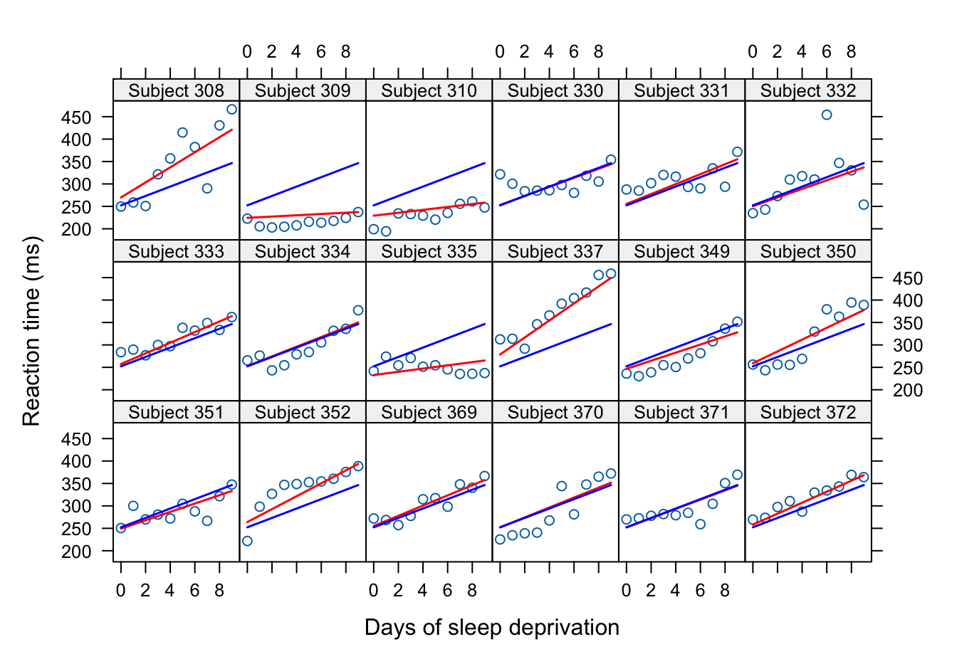
Figure 31.2 displays the population-average and subject-specific predictions of the reaction times for all 18 subjects. The population-average trend (blue) is the same in all panels. The subject-specific trends vary from panel to panel. Subject 330 behaves very much like the population average. Subject 337 has a very different slope, their reaction time increases much more quickly than that of the average subject. The linear mixed model with autocorrelated error captures a remarkable degree of variability, based on only seven parameters.
xyplot(Reaction ~ Days | Subject, data=sleepstudy,xlab="Days of sleep deprivation",ylab="Reaction time (ms)",type=c("p"),as.table=TRUE,layout=c(6,3,1),panel=function(x,y,...) { grpname <-dimnames(trellis.last.object())[[1]][packet.number()]panel.xyplot(x,y,...)panel.lines(x,predvals$predict.Sub[predvals$Sub == grpname],col="red",lwd=1.5)panel.lines(x,predvals$predict.fixed[predvals$Sub == grpname],col="blue",lwd=1.5) },strip =function(...) {strip.default(..., strip.names =TRUE, strip.levels=TRUE,sep=" ") },par.strip.text =list(cex =0.8), )
Figure 31.2: Population-average (blue) and subject-specific (red) predictions in sleep study.
31.3 Generalized Linear Mixed Models (GLMM)
Introduction
The transition from the classical linear model to generalized linear models (GLM) in Chapter 28 added to the linear model
that the distribution of \(Y\) is a member of the exponential family of distributions
an invertible link function \(g(\mu)\) that maps between the scale of the data (the scale of the response) and the input variables.
Common to both model families is to express the effect of the input variables through a linear predictor \[
\eta = \textbf{x}^\prime \boldsymbol{\beta}
\] A GLM, written in vector form, can thus be summarized as follows: \[
\begin{align*}
Y &\sim P_{expo} \\
\text{E}[Y] &= \mu(\boldsymbol{\beta}) \\
g(\mu) &= \eta \\
\eta &= \textbf{x}^\prime\boldsymbol{\beta}
\end{align*}
\]
The extension to a mixed-model version, the generalized linear mixed model (GLMM) seems obvious: extend the linear predictor with random variables \(\textbf{b}\): \[
\begin{align*}
Y | \textbf{b}&\sim P_{expo} \\
g(\mu) &= \textbf{x}^\prime\boldsymbol{\beta}+ \textbf{z}^\prime \textbf{b}\\
\eta &= \textbf{x}^\prime\boldsymbol{\beta}+ \textbf{z}^\prime \textbf{b}
\end{align*}
\] where \(\textbf{b}\) follows some distribution, a \(G(\textbf{0},\textbf{G})\), say. Similar to the GLM and the LMM, we then estimate the parameters based on maximizing the log likelihood of the marginal distribution of \(Y\).
This works well on paper!
Compared to the linear mixed model, where \(\textbf{b}\) and \(Y\) followed a Gaussian distribution and deriving the marginal distribution of \(Y\) is straightforward, the same is not true for the GLMM family of models. Here are some of the complications we run into:
The marginal distribution of \(Y\) is obtained by integrating over the distribution of the random effects, \[
p(y) = \int \cdots \int p(y|\textbf{b}) p(\textbf{b}) \, d\textbf{b}
\]\(p(y)\) does not generally have a closed form (as in the Gaussian-Gaussian case) and this multidimensional integral must be computed by numerical methods.
A valid joint distribution of the data might not actually exist. Gilliland and Schabenberger (2001) show, for example, that if \(\textbf{Y}\) is an \((n\times 1)\) vector of equicorrelated binary variables with common success probability \(\pi\), then the lower bound of the correlation parameter depends on \(n\) and \(\pi\). In other words, if you obtain an estimate of the correlation parameter that falls below that lower bound, there is no probability model that could have possibly generated the data.
The incorporation of correlated errors with or without the presence of random effects in the model is questionable when data do not follow a Gaussian distribution. Achieving desired properties of the marginal distribution and the conditional distribution might not be possible if the data are non-Gaussian.
Because the marginal distribution is difficult to come by, population-average inference is difficult in GLMM; we do not know the functional form of the marginal mean. The obvious attempt to simply evaluate the inverse link function at the mean of the random effects, \[
g^{-1}(\textbf{x}^\prime\boldsymbol{\beta}+ \textbf{z}^\prime\text{E}[\textbf{b}]) = g^{-1}(\textbf{x}^\prime\boldsymbol{\beta}+ 0) = g^{-1}(\textbf{x}^\prime\boldsymbol{\beta})
\] does not yield the estimate of the marginal mean. Predictions in GLMMs thus focus on the conditional mean, \(\mu|\textbf{b}= g^{-1}(\textbf{x}^\prime\boldsymbol{\beta}+ \textbf{z}^\prime\textbf{b})\). In longitudinal studies, this is the cluster-specific mean.
In short, training generalized linear mixed models is much more complicated than working with their linear counterpart, and we typically have to restrict the types of models under consideration somehow.
Estimation Approaches
The approaches to estimating parameters in GLMMs fall broadly into two categories:
Linearization methods approximate the model based on Taylor series. Similar to fitting a nonlinear or generalized linear model as a series of approximate linear models based on a vector of pseudo data, these methods approximate the GLMM through a series of LMMs. The advantage of the linearization methods is that the approximate LMM can accommodate complex random effects structures and correlated errors. There is no limit to the types of covariance structure you can specify with this approach. The disadvantages of linearization are the absence of a true objective function, the log likelihood of \(Y\) is never calculated, the estimates are not maximum likelihood estimates, and they are often biased.
Integral approximation methods compute the log likelihood using numerical techniques such as Laplace approximation, Gauss-Hermite quadrature, Monte Carlo integration and other methods. The advantage of this approach is that the log likelihood of \(Y\) is being computed and maximum likelihood estimates are obtained. The disadvantage is the computational demand, increasing quickly with the number of random effects and the number of abscissas in the integral approximation. Integral approximations are thus used for relatively simple models that have only few random effects.
The Laplace and Gauss-Hermite quadrature integral approximations are related. The former is a Gauss-Hermite quadrature with a single quadrature node. The marginal joint distribution of the data in a mixed model is \[
\begin{align*}
p(\textbf{y}) &= \int \cdots \int p(\textbf{y}| \textbf{b}, \boldsymbol{\beta}) p(\textbf{b}| \boldsymbol{\theta}) \, d\textbf{b}\\
&= \int \cdots \int \exp\{c f(\textbf{y},\boldsymbol{\beta},\boldsymbol{\theta},\textbf{b}\} \, d\textbf{b}
\end{align*}
\] for some function \(f()\) and constant \(c\). If \(c\) is large, the Laplace approximation of \(p(\textbf{y})\) is \[
\left(\frac{2\pi}{c} \right)^{n_b/2} |-f^{\prime\prime}(\textbf{y}, \boldsymbol{\beta},\boldsymbol{\theta},\tilde{\textbf{b}})|^{-1/2}\exp\left\{cf(\textbf{y},\boldsymbol{\beta},\boldsymbol{\theta},\textbf{b})\right\}
\] where \(f^{\prime\prime}\) is the second derivative of \(f\) evaluated at \(\tilde{\textbf{b}}\) at which \(f\) has a minimum. This looks like a messy expression and requires a sub-optimization to find \(\tilde{\textbf{b}}\) such that \(f^\prime(\textbf{y},\boldsymbol{\beta},\boldsymbol{\theta},\tilde{\textbf{b}})=0\), but it is simpler than computing the integral by other means. The Laplace approximation is thus a common method to solving the maximum likelihood problem in GLMMs.
With longitudinal data, the quality of the Laplace approximation increases with the number of clusters and the number of observations within a cluster.
GLMM in R
The glmer function in the lme4 package fits generalized linear mixed models by adaptive gaussian quadrature and Laplace approximation for relatively simple random effects structures.
Example: Contagious Bovine Pleuropneumonia
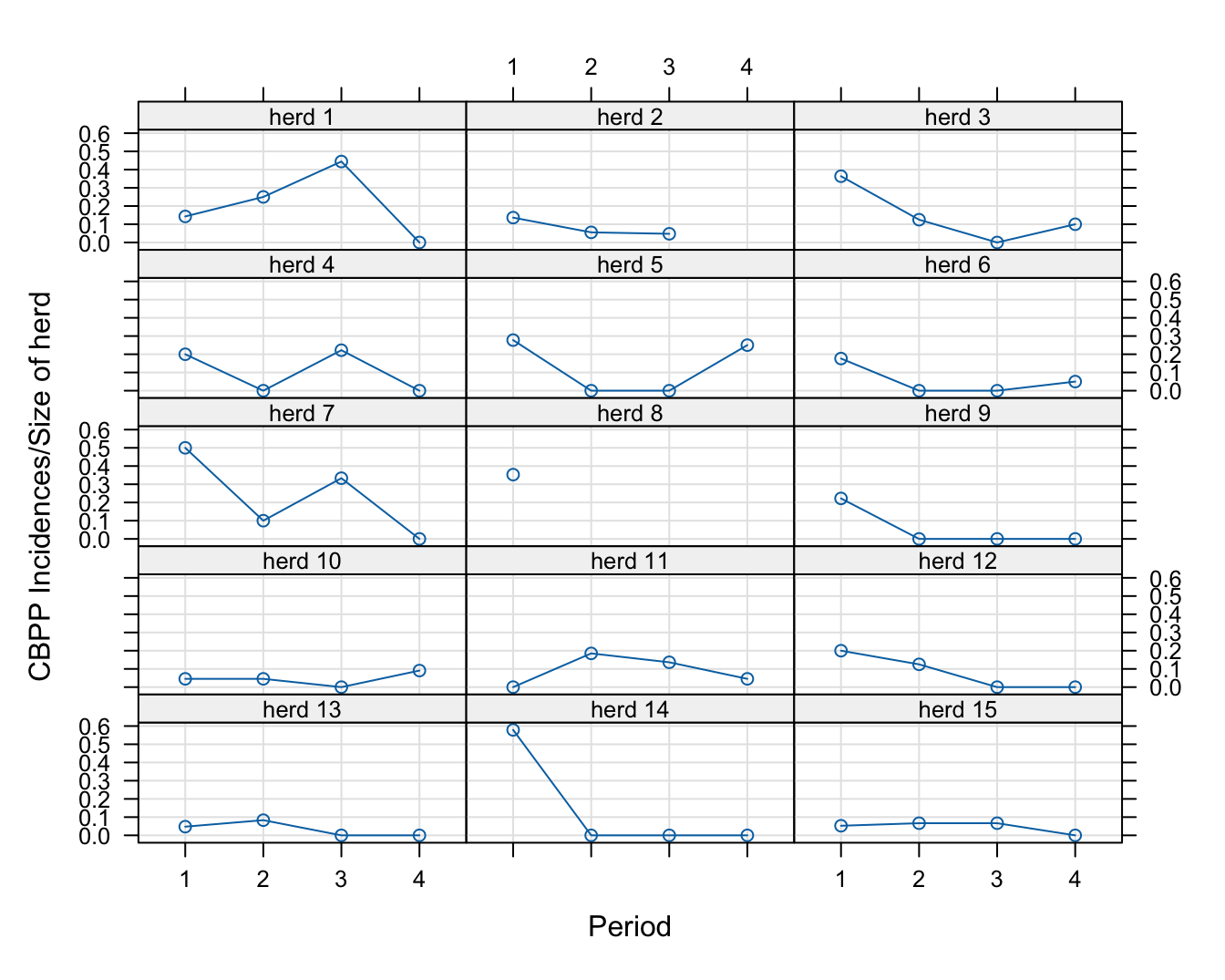
The data set cbpp comes with the lme4 library and contains serological incidences of contagious bovine pleuropneumonia (CBPP) in 15 commercial cattle herds in Africa. Blood samples were collected quarterly from the animals of each herd. The data were used to compute the new cases that occurred during the time period.
There are 56 observations for the 15 herds. The outcome of interest is the number of incidences in the herd, a Binomial random variable. Figure 31.3 shows a trellis plot of the incidence proportions over time for each herd.
Generalized linear mixed model fit by maximum likelihood (Laplace
  Approximation) [glmerMod]
 Family: binomial  ( logit )
Formula: cbind(incidence, size - incidence) ~ as.numeric(period) + (1 |
    herd)
   Data: cbpp

      AIC       BIC    logLik -2*log(L)  df.resid
    192.6     198.6     -93.3     186.6        53

Scaled residuals:
    Min      1Q  Median      3Q     Max
-2.2566 -0.7991 -0.4361  0.5804  3.0664

Random effects:
 Groups Name        Variance Std.Dev.
 herd   (Intercept) 0.4402   0.6635
Number of obs: 56, groups:  herd, 15

Fixed effects:
                   Estimate Std. Error z value Pr(>|z|)
(Intercept)         -0.9323     0.3017  -3.090    0.002 **
as.numeric(period)  -0.5592     0.1219  -4.589 4.46e-06 ***
---
Signif. codes:  0 '***' 0.001 '**' 0.01 '*' 0.05 '.' 0.1 ' ' 1

Correlation of Fixed Effects:
            (Intr)
as.nmrc(pr) -0.721
The estimates of the fixed effects are \(\widehat{\boldsymbol{\beta}}\) = [-0.9323, -0.5592]. The variance of the herd-specific random intercept is \(\text{Var}[b_0]\) = 0.4402.
The sum of the fixed and random coefficients for each level of the subject variable can be accessed with the coef function:
The model with a random slope adds two parameters, the variance of the random slope, \(\sigma^2_1\) and the covariance between random intercept and random slope,\(\sigma_{01}\). The LRT has a test statistic of 2.3946 with \(p\)-value of 0.302. The addition of the random slope does not significantly improve the model; we stick with the random intercept model.
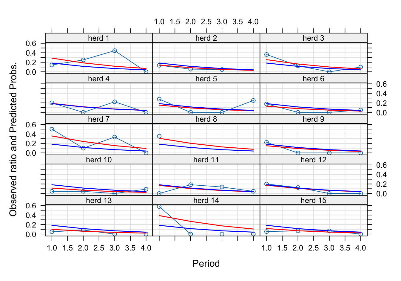
Figure 31.4 shows the predicted probabilities along with the observed incidence ratios for each herd. These predictions on the scale of the data (the probability scale) are obtained with
re.form=NULL adds all random effects in the linear predictor, re.form=NA sets the random effects to zero.
The blue line is the “population average” which is the predicted value on the data scale obtained by setting the random effects to zero. This is not an unbiased estimate of the incidence probability of the average herd. The linear trend in observation period on the logit scale maps to a nonlinear trend on the probability scale.
Notice that predicted values can be computed for all periods, even if a herd was measured during only some periods. For example, herd #8 was observed only once, but a subject-specific prediction is possible for all periods because a subject-specific intercept \(\widehat{b}_{0(8)}\) is available.
Figure 31.4: “Population-average” (blue) and subject-specific (red) predictions in CBPP study.
Belenky, Gregory, Nancy J. Wesensten, David R. Thorne, Maria L. Thomas, Helen C. Sing, Daniel P. Redmond, Michael B. Russo, and Thomas J. Balkin. 2003. “Patterns of Performance Degradation and Restoration During Sleep Restriction and Subsequent Recovery: A Sleep Dose-Response Study.”Journal of Sleep Research 12: 1--12.
Gilliland, D., and O. Schabenberger. 2001. “Limits on Pairwise Association for Equi-Correlated Binary Variables.”Journal of Applied Statistical Sciences 10: 279--285.
Harville, D. A. 1976. “Extension of the Gauss-Markov Theorem to Include the Estimation of Random Effects.”The Annals of Statistics 4: 384–95.
Henderson, C. R. 1950. “The Estimation of Genetic Parameters.”The Annals of Mathematical Statistics 21 (2): 309–10.
———. 1984. Applications of Linear Models in Animal Breeding. University of Guelph.