library(duckdb)

con <- dbConnect(duckdb(),dbdir="ads.ddb", read_only=FALSE)
simReg <- dbGetQuery(con,"SELECT * from SiMRegData;")
dbDisconnect(con)11 Local Models
In Chapter 6 we introduced different approaches to structure the problem of finding \[ \text{E}[Y_i | \textbf{x}_i] = f^*(\textbf{x}_i) \] by constraining the model family or the estimation approach. Section 6.2 then introduced the concept of global and local models.
The methods discussed in this part of the book so far are global models in the sense that they depend on parameters \(\boldsymbol{\beta}\) that apply regardless of the position \(\textbf{x}_0\) in the regression hull. Global models do not have a different set of parameters at \(\textbf{x}_i\) and \(\textbf{x}_j\).
In this chapter we discuss in greater detail models that capture local variations of the mean function. The two major approaches to give models greater flexibility is through the introduction of weight functions or through basis expansions. Kernel regression and local polynomials are examples of the weighting approach. Regressions and smoothing splines are examples of the basis expansion approach.
Because these methods suffer from the curse of dimensionality (Section 6.4.1), they are not applied in higher dimensions. For the remainder of this chapter we assume a single input variable, \(\textbf{x}= x\).
11.1 Kernel Regression
A special case of a kernel regression estimator was introduced in Section 6.4, the \(k\)-nearest neighbor regression estimator. The idea is simple: to predict the mean of \(Y\) at \(x_0\), find the \(k\) observations closest to \(x_0\) and take their average. The procedure can be formalized as follows:
The general model is \(Y(x) = f(x) + \epsilon\) with \(\text{E}[\epsilon] = 0\)
To predict \(f(x_0)\) use the local estimator \(\widehat{f}(x_0) = \frac{1}{k}\sum_{i=1}^k y(x_{(i)})\) where \(x_{(i)}\) is the \(i\)th closest observation to \(x_0\) and \(y(x_{(i)})\) is the observed value of the target variable at \(x_{(i)}\).
This is equivalent to considering at \(x_0\) the regression model \[ Y(x_0) = \beta + \epsilon^* \] in just a neighborhood of \(x_0\). This is an intercept-only model and the OLS estimator is \(\widehat{\beta} = \overline{y}\). To make it so the model uses only the \(k\) observations closest to \(x_0\) we fit it as a weighted regression. The weight of an observation is 1 if it is within the \(k\)-neighborhood and 0 if it is outside. Formally, the weight function at \(x_0\) is
\[ K(x_0,x_i) = I(||x_i-x_0|| \le ||x_{(k)} - x_0 ||) \] where \(x_{(k)}\) denotes the observation ranked \(k\)th in distance from \(x_0\), \(||x_i-x_0||\) denotes the distance of \(x_i\) from the prediction location \(x_0\), and \(I()\) is the indicator function (\(I(a)\) is 1 if \(a\) is true).
- When the weight function is applied, the estimator of \(\beta\) becomes \[ \widehat{\beta}(x_0) = \frac{\sum_{i=1}^n K(x_0,x_i) \, y(x_i)}{\sum_{i=1}^n K(x_0,x_i)} = \frac{1}{k}\sum_{i=1}^k y(x_{(i)}) \]
What have we accomplished with this setup? A global model, \(Y(x) = \beta + \epsilon^*\), which is probably not correct over the range of \(X\) has turned into a local model for \(Y(x_0)\) by introducing a weight function that gives more weight to observations close to \(x_0\) than to observations far away. It is much more reasonable to assume an intercept-only model holds at \(x_0\) than across the entire range of \(X\). As the prediction problem moves to another location, say \(x^*_0\), the weighted regression problem is solved again, this time based on the weight function \[ K(x^*_0,x_i) = I(||x_i-x^*_0|| \le ||x_{(k)} - x^*_0 ||) \]
Rather than one global estimate \(\widehat{\boldsymbol{\beta}}\) we get as many estimates as there are points we wish to predict at: \(\widehat{\beta}(x_0), \widehat{\beta}(x^*_0), \widehat{\beta}(x^{**}_0), \cdots\).
The data shown in Figure 11.1 is simulated according to a data set in the course on Predictive Modeling by García-Portugués (2024). The true mean function is \[ f(x) = x^2 \, \cos(x) \] and the observed data (Figure 11.1) follow the model \[ Y(x) = f(x) + \epsilon\quad \epsilon \sim \textit{iid } G(0,4) \]
import duckdb
import pandas as pd

con = duckdb.connect(database="ads.ddb", read_only=True)
simReg = con.sql("SELECT * FROM SimRegData;").df()
con.close()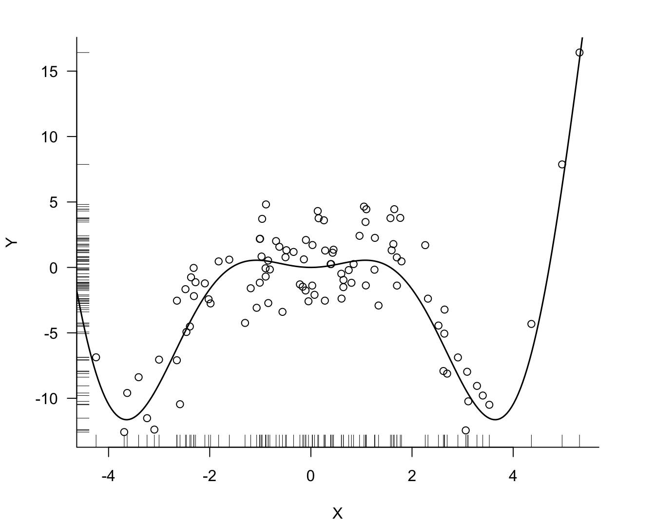
Example: 3-nearest Neighbor Estimation
The following code computes the 3-NN regression estimator at a grid of \(x_0\) values, ranging from -4 to 4.
x_0 <- seq(-4,4,1)
k3_reg <- Rfast::knn(as.matrix(x_0),
                     as.matrix(simReg$Y),
                     as.matrix(simReg$X),k=3,type="R")

cbind(x_0,k3_reg)
x_0
[1,] -4 -9.681715
[2,] -3 -10.319916
[3,] -2 -2.134633
[4,] -1 1.066642
[5,] 0 -0.755860
[6,] 1 3.510851
[7,] 2 1.982169
[8,] 3 -9.101672
[9,] 4 -8.201705The same results can be obtained using an intercept-only model with weights calculated according to \(K(x_0,x_i)\). The proxy::dist() function computes the distance between the \(x_0\) locations and the \(x\) values. The loop constructs the weight vector for each prediction point, assigning 1 to the points within the 3-neighbor distance and 0 to the points outside. The only change in the call to lm() from one prediction point to the next is the vector of weights.
d <- proxy::dist(x_0,simReg$X,method="euclidean")
for (i in 1:length(x_0)) {
    d_lim <- head(sort(d[i,]),3)
    w <- rep(0,length(simReg$X))
    w[which((d[i,] >= d_lim[1] & (d[i,] <= d_lim[3])))] <- 1
    cat("x_0: ", x_0[i], "beta_hat: ",lm(simReg$Y ~ 1, weights=w)$coefficients,"\n")
}
x_0: -4 beta_hat: -9.681715
x_0: -3 beta_hat: -10.31992
x_0: -2 beta_hat: -2.134633
x_0: -1 beta_hat: 1.066642
x_0: 0 beta_hat: -0.75586
x_0: 1 beta_hat: 3.510851
x_0: 2 beta_hat: 1.982169
x_0: 3 beta_hat: -9.101672
x_0: 4 beta_hat: -8.201705 import numpy as np
from sklearn.neighbors import KNeighborsRegressor
x_0 = np.arange(-4, 5, 1)
x_0_reshaped = x_0.reshape(-1, 1)
knn = KNeighborsRegressor(n_neighbors=3)
knn.fit(np.array(simReg.X).reshape(-1,1), np.array(simReg.Y).reshape(-1,1))KNeighborsRegressor(n_neighbors=3)In a Jupyter environment, please rerun this cell to show the HTML representation or trust the notebook.
On GitHub, the HTML representation is unable to render, please try loading this page with nbviewer.org.
KNeighborsRegressor(n_neighbors=3)
k3_reg = knn.predict(x_0_reshaped)

result = np.column_stack((x_0, k3_reg))
print(result)
[[ -4. -9.68171548]
[ -3. -10.31991643]
[ -2. -2.13463283]
[ -1. 1.06664192]
[ 0. -0.75585997]
[ 1. 3.51085137]
[ 2. 1.98216901]
[ 3. -9.10167227]
[ 4. -8.20170506]]The same results can be obtained using an intercept-only model with weights calculated according to \(K(x_0,x_i)\). The cdist function computes the distance between the \(x_0\) locations and the \(x\) values. The loop constructs the weight vector for each prediction point, assigning 1 to the points within the 3-neighbor distance and 0 to the points outside. The only change in the call to the weighted least squares function sm.WLS is the change in the weight vector between the prediction points.
import numpy as np
from scipy.spatial.distance import cdist
from sklearn.linear_model import LinearRegression
import statsmodels.api as sm

Y = np.array(simReg.Y).reshape(-1,1)
X = np.array(simReg.X).reshape(-1,1)

# Calculate Euclidean distance matrix
d = cdist(x_0_reshaped, X, metric='euclidean')

for i in range(len(x_0)):
    distances = d[i, :]
    sorted_indices = np.argsort(distances)

    # Get the 3 closest distances
    d_lim = distances[sorted_indices[:3]]

    w = np.zeros(len(X))
    # Set weight to 1 for points with distances between d_lim[0] and d_lim[2] (inclusive)
    mask = (distances >= d_lim[0]) & (distances <= d_lim[2])
    w[mask] = 1

    # Fit weighted linear model with intercept only (Y ~ 1)
    model = sm.WLS(Y, np.ones(len(Y)), weights=w)
    results = model.fit()

    print(f"x_0: {x_0[i]}, beta_hat: {results.params[0]:.4f}")
x_0: -4, beta_hat: -9.6817
x_0: -3, beta_hat: -10.3199
x_0: -2, beta_hat: -2.1346
x_0: -1, beta_hat: 1.0666
x_0: 0, beta_hat: -0.7559
x_0: 1, beta_hat: 3.5109
x_0: 2, beta_hat: 1.9822
x_0: 3, beta_hat: -9.1017
x_0: 4, beta_hat: -8.2017Nadaraya-Watson Estimator
The previous estimator is a special case of the Nadaraya-Watson kernel estimator of \(f(x_0)\), \[ \widehat{f}(x_0) = \frac{\sum_{i=1}^n K_\lambda(x_0,x_i)\,y_i}{\sum_{i=1}^nK_\lambda(x_0,x_i)}=\sum_{i=1}^n w_i(x_0)\,y_i \]
The expression on the right shows that this is a weighted estimator where the weights are given by \[ w_i(x_0) = \frac{K_\lambda(x_0,x_i)}{\sum_{i=1}^n K_\lambda(x_0,x_i)} \] The kernel function \(K_\lambda(x_0,x_i)\) depends on the prediction location \(x_0\), the distance \(|x_i-x_0|\) between \(x_i\) and \(x_0\), and a parameter \(\lambda\) that controls the shape of the kernel. \(\lambda\) is called the bandwidth of the kernel because it controls how quickly the kernel weights drop with increasing distance from \(x_0\); or in other words, how wide the kernel function is.
Popular kernel functions are
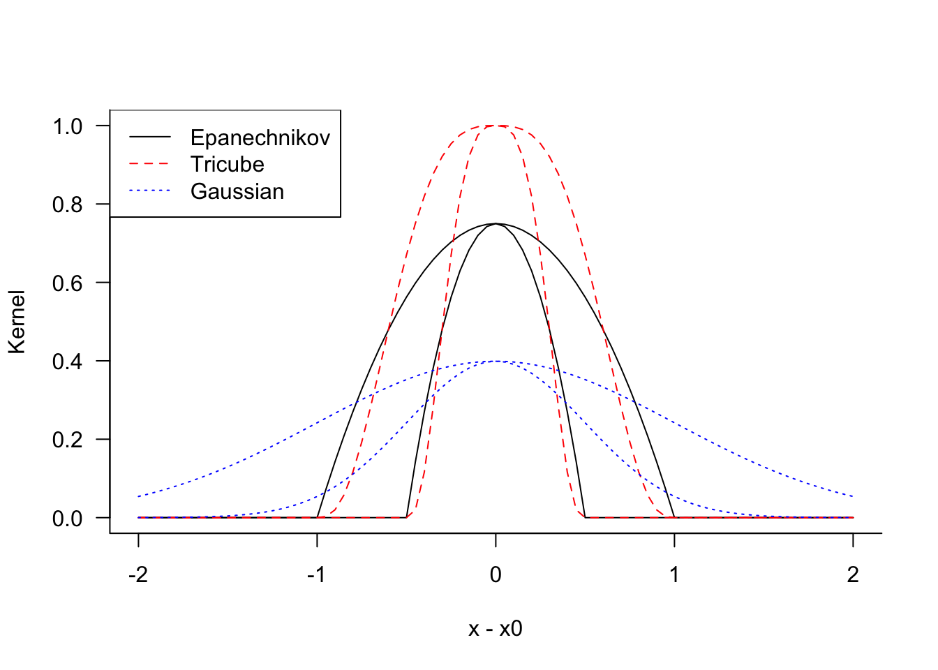
Epanechnikov kernel \[ K_\lambda(x_0,x) = \left \{ \begin{array}{ll} \frac{3}{4}\left(1-t^2\right) & \text{if } |t| \le 1 \\ 0 & \text{otherwise} \end{array}\right . \]
Tricube kernel \[ K_\lambda(x_0,x) = \left \{ \begin{array}{ll} \frac{3}{4}\left(1-|t|^3\right)^3 & \text{if } |t| \le 1 \\ 0 & \text{otherwise} \end{array}\right . \]
Gaussian kernel \[ K_\lambda(x_0,x) = \phi(t) \]
In these expressions \(t = |x - x_0|/\lambda\) and \(\phi(t)\) is the standard Gaussian density function.
Figure 11.2 shows the kernel functions for \(\lambda=0.5\) and \(\lambda=1\), respectively. The functions reach their maximum at \(|x-x_0| = 0\) and decrease symmetrically in both directions. The Epanechnikov has a kink at \(|t| = \lambda\) while the tricube kernel transitions smoothly through that point. Tricube kernels are sometimes preferred over the Epanechnikov kernel because the latter is not differentiable at \(|t|=1\). The Gaussian kernel is very smooth and for a given value of \(\lambda\) assigns greater weights for points remote from \(x_0\).
In practice, the choice of the kernel function is less important than the choice of the bandwidth parameter \(\lambda\).
Example: Kernel Regression with Simulated Data
The ksmooth() function in the stats package (built-in) can be used to compute the kernel regression smoother. x.points= specifies the points at which to evaluate the smoothed fit. kernel="normal" chooses the Gaussian kernel.
You can also use the locpoly function in the KernSmooth package, an example follows later.
kr_05 <- ksmooth(simReg$X,simReg$Y,kernel="normal",bandwidth=0.5, x.points=xGrid)
kr_09 <- ksmooth(simReg$X,simReg$Y,kernel="normal",bandwidth=0.9, x.points=xGrid)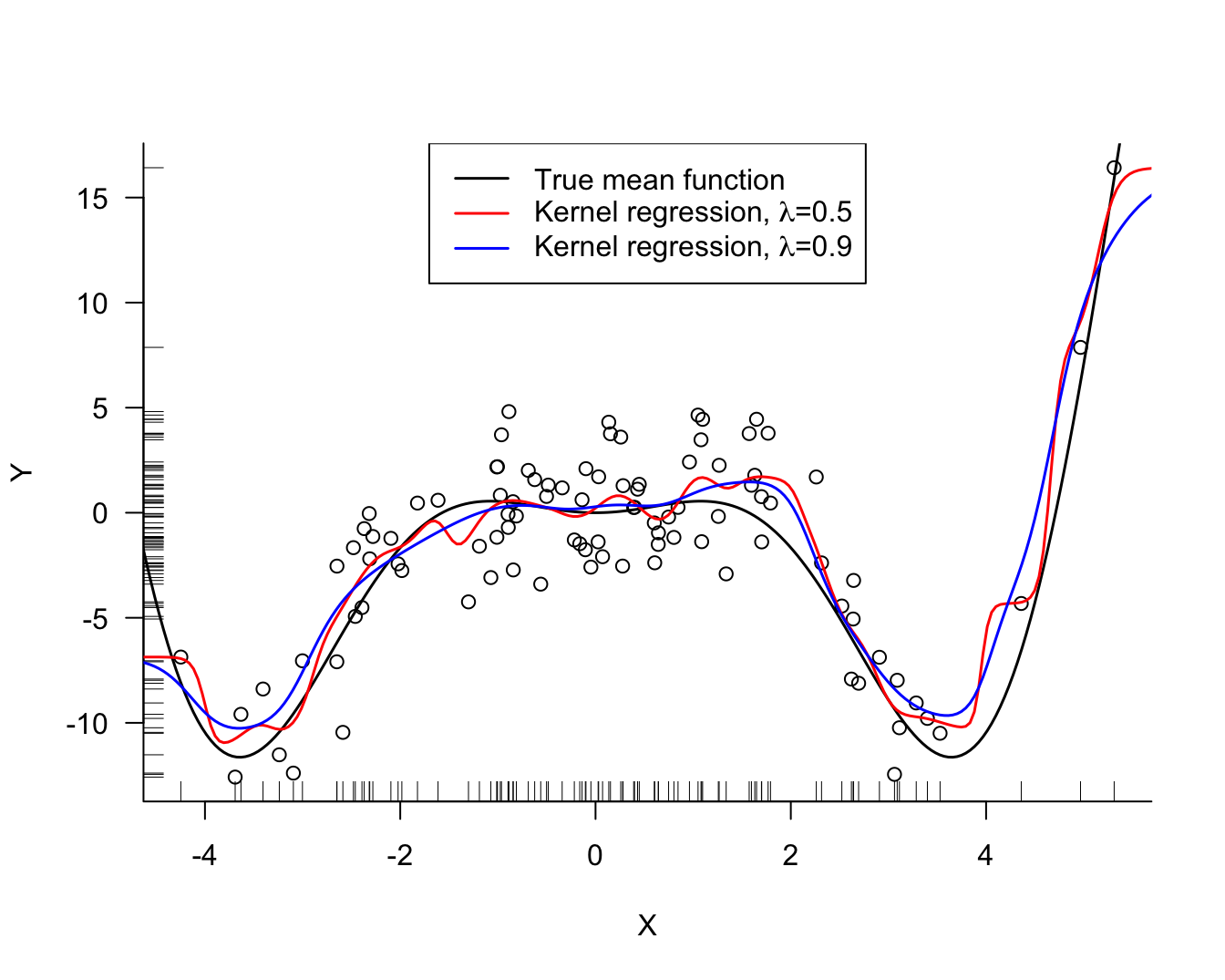
The KernelReg function in statsmodels computes the kernel regression smoother. By default the function fits local linear regression models with a Gaussian kernel. The var_type='c' parameter instructs the function that the variables in the model are continuous. To match the results of the kernel regression smoother ksmooth() in R, we set reg_type='lc' to request a local constant model.
from statsmodels.nonparametric.kernel_regression import KernelReg
X = np.array(simReg.X).flatten()
Y = np.array(simReg.Y).flatten()

xGrid = np.linspace(-5, 6, 250)
xGrid = np.array(xGrid).flatten()

def m(x):
    return x**2 * np.cos(x)

kr_model_1 = KernelReg(endog=Y, exog=X, var_type='c', reg_type='lc',bw=[0.186])
kr_1_mean, kr_1_mfx = kr_model_1.fit(xGrid)

kr_model_2 = KernelReg(endog=Y, exog=X, var_type='c', reg_type='lc', bw=[0.33])
kr_2_mean, kr_2_mfx = kr_model_2.fit(xGrid)
(-14.032172932031724, 20.0)
Several noteworthy items in Figure 11.3:
The kernel regression estimate for larger values of \(\lambda\) is more smooth than the estimate for smaller values of \(\lambda\). A larger bandwidth widens the kernel (weight) function. As \(\lambda\) increases the fit approaches a flat line at \(\widehat{\beta} = \overline{y}\), a global model.
In contrast to the \(k\)-NN estimator, the kernel regression estimator is smooth. \(k\)-NN estimates change abruptly when a point leaves the \(k\)-neighborhood and another point enters. The \(k\)-NN weight function \[ K(x_0,x_i) = I(||x_i-x_0|| \le ||x_{(k)} - x_0 ||) \] is not smooth. The weight associated with a data point \(x_i\) in kernel regression changes gradually with its distance from \(x_0\).
Fitting the model at \(x_0\) and predicting at \(x_0\) is the same operation; unlike in global models where you fit the model first, obtain the parameters, and then use them to predict at any point you choose.
There must be a variance-bias tradeoff between the bias of a model with large bandwidth and the variability of a model with small bandwidth. The hyperparameter \(\lambda\) can be chosen by some form of cross-validation.
The kernel regression estimates generally capture the mean function well, but seem to struggle near the edges of the \(x\)-range. Both underestimate the trend at the edge, the estimate for small \(\lambda\) turns away more sharply than the estimate for the larger \(\lambda\) value. The problem near the edge is that the estimator can use information only from one side of the edge. Fitting the model at \(x_0 = \max(x_i)\) only observations with \(x < x_0\) are assigned non-zero weight. Unless the mean function is flat beyond the range of \(x\), the kernel estimator will be biased near the edges of the range.
Note
If you compare the R and Python results in the previous example, it appears that the ksmooth and KernelReg functions arrived at the same fits for different values of the bandwidth parameter, \([0.5, 0.9]\) in R and \([0.186, 0.33]\) in Python.
The reason for the discrepancy is thatksmooth in R uses the bandwidth parameter to scale the Gaussian kernel so that the first and third quartiles are at \(\pm 0.25 \lambda\). The inter-quartile range of the Gaussian distribution is approximately 1.34 times its standard deviation.
The KernelReg function uses the bandwidth as the standard deviation of the Gaussian kernel (I think!). The value \(\lambda=0.9\) in ksmooth places the quartiles at \(\pm 0.225\), the inter-quartile range is 0.45 and the corresponding standard deviation of the Gaussian kernel in kmsooth is \(0.45/1.34 = 0.33\).
Cross-validation for \(\lambda\)
The best value for \(\lambda\) that resolves the bias-variance tradeoff for a particular set of data can be determined by a form of cross-validation.
Example: Kernel Regression with Simulated Data
The ksmooth function in R does not support cross-validation so we implement a function from scratch for LOOCV based on the average squared prediction residual (PRESS). The function is then evaluated on a grid of candidate bandwidth values. For each value of the bandwidth, every data point is removed from the training set, then predicted, and its contribution to the prediction sum of squares is calculated.
ksm.cv <- function(X,Y,bw=0.5) {
MSTe <- rep(0,length(bw))
for (j in seq_along(bw)) {
PRESS <- 0
ngood <- 0
for (i in seq_along(X)) {
nw <- ksmooth(x =X[-i],
y =Y[-i],
kernel ="normal",
bandwidth=bw[j],
x.points =X[i])
if (!is.na(nw$y)){
PRESS <- PRESS + (Y[i] - nw$y)^2
ngood <- ngood + 1
}
}
MSTe[j] = PRESS/ngood
}
return (as.data.frame(cbind(bw,MSTe,ngood)))
}
bw_grid <- seq(0.5,1.5,0.01)
cvres <- ksm.cv(simReg$X,simReg$Y,bw_grid)
cat("Smallest LOOCV MSE ",
cvres$MSTe[which.min(cvres$MSTe)],
" at bandwidth ",
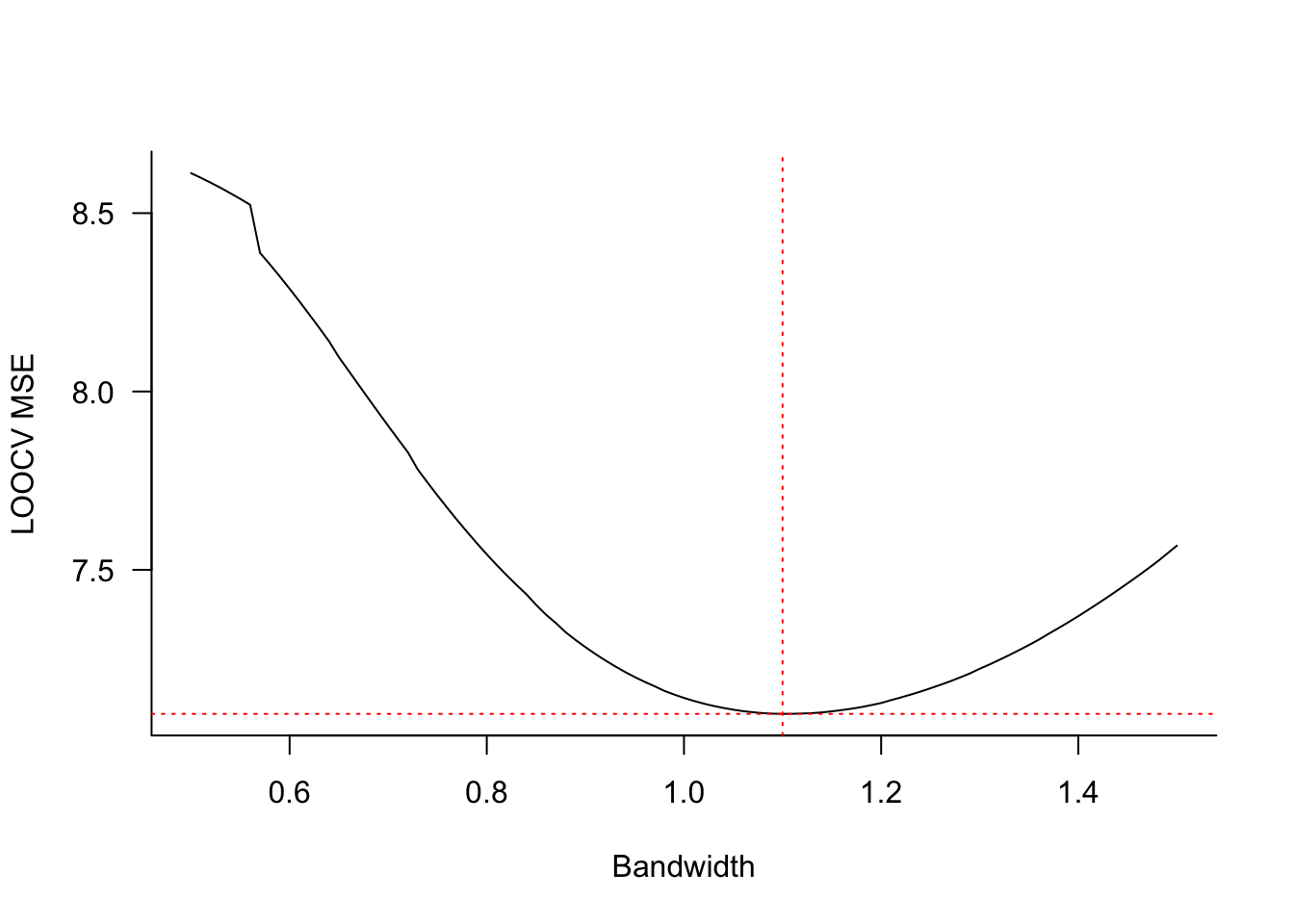
cvres$bw[which.min(cvres$MSTe)])Smallest LOOCV MSE 7.09627 at bandwidth 1.1Figure 11.4 displays the LOOCV mean-squared error for bandwidth values from 0.5 to 1.5 in steps of 0.01. The smallest error is achieved at \(\lambda = 1.1\). Figure 11.5 displays the kernel regression estimate for that bandwidth. The local model fits the data well but continues to show bias at the boundary of the \(x\)-range.

In Python we can rely on the built-in cross-validation of the KernelReg function in statsmodels to determine the best bandwidth by leave-one-out cross-validation. To trigger cross-validation, either pass an array of bandwidth values in the bw argument or specify bw='cv_ls'.
from statsmodels.nonparametric.kernel_regression import KernelReg

X = np.array(simReg.X).flatten()
Y = np.array(simReg.Y).flatten()

xGrid = np.linspace(-5, 6, 250)
xGrid = np.array(xGrid).flatten()

kr_model = KernelReg(endog=Y, exog=X, var_type='c',reg_type='lc',bw='cv_ls')
kr_mean, kr_mfx = kr_model.fit(xGrid)

print(f"Cross-validated bandwidth: {kr_model.bw[0]:.4f}")
Cross-validated bandwidth: 0.4093Figure 11.6 displays the kernel regression estimate for the selected bandwidth of 0.4093. The local constant model fits the data well but continues to show bias at the boundary of the \(x\)-range.
(-14.032172932031724, 20.0)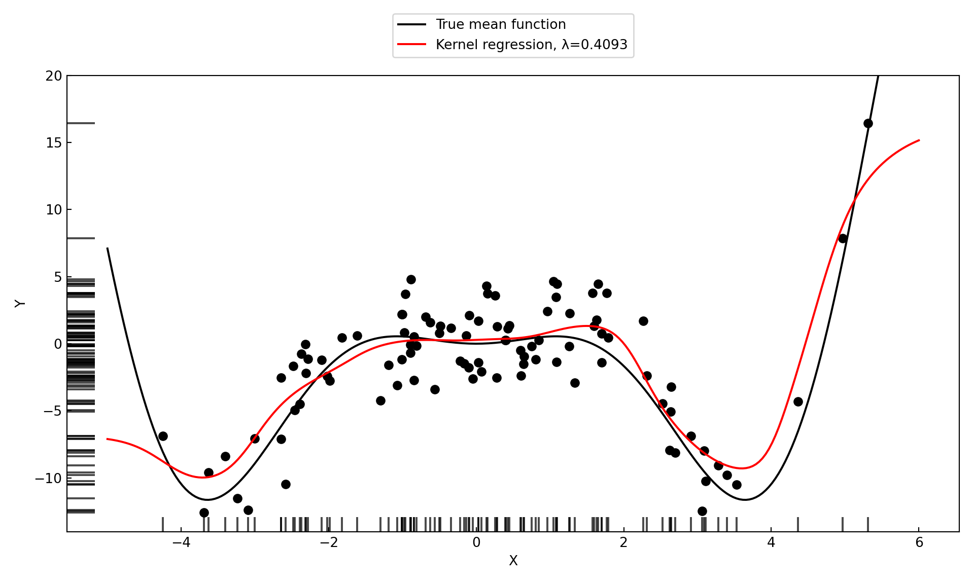
Tip
When you graph the results of cross-validation and the minimum criteria is achieved for the smallest (or largest) value of the hyperparameter being validated, you need to extend the grid of values below (or above) the values considered. Otherwise you might erroneously conclude that the “best” value is the value on the boundary of your candidate values. This is not a problem in Figure 11.4 where the minimum MSE does not fall on the boundary.
11.2 Local Regression
The kernel regression estimate at \(x_0\) is equivalent to fitting a weighted intercept-only model \[ Y(x) = \beta_0 + \epsilon \] where the weights are calculated according to a kernel function with some bandwidth \(\lambda\): \[ w_i(x_0) = \frac{K_\lambda(x_0,x_i)}{\sum_{i=1}^n K_\lambda(x_0,x_i)} \]
Local regression generalizes this idea to weighted polynomial regression models. A local regression model of degree 1 (linear) is a weighted regression with mean function \[ Y(x) = \beta_0 + \beta_1 x + \epsilon \] A local regression model of degree 2 (quadratic) is a weighted regression with mean function \[ Y(x) = \beta_0 + \beta_1 x + \beta_2 x^2 + \epsilon \] and so on. The kernel regression estimate of the previous section is a special case, a local regression model of degree 0.
The parameters in the local regression model change with prediction location \(x_0\) because the kernel weight function changes with \(x_0\). Formally, the estimates at \(x_0\) satisfy a weighted least squares criterion. For a model of degree 1 the criterion is
\[ \mathop{\mathrm{arg\,min}}_{\beta_0(x_0), \beta_1(x_0)} = \sum_{i=1}^n K_\lambda(x_0,x_i) \left(y_i - \beta_0(x_0) - \beta_1(x_0) x_i \right )^2 \]
Choosing the Degree
The degree of a local regression polynomial is typically small, \(p=1\) or \(p=2\). Higher-order polynomials are against the principle of local methods to approximate any function by a low-order polynomial in a small neighborhood .
The boundary bias we noticed in the kernel regression (\(p=0\)) estimates is greatly reduced when \(p > 0\). The local model now depends on \(x\) and does not approximate the mean with a flat line near the boundary.
For the same bandwidth, a quadratic model will be more flexible (wiggly) than a linear model. With curved trends, quadratic models can fit better than linear models in the interior of the \(x\) range. This is a classical bias-variance tradeoff.
Example: Linear and Quadratic Local Polynomials with Simulated Data
The KernSmooth::locpoly function in R computes local polynomial regression estimates with Gaussian kernels. For comparison purposes, the following code fit models of degree 0, 1, and 2 with the same bandwidth. For degree 0 we get the Nadaraya-Watson kernel regression estimator. For degree 1 we are fitting a local linear regression, for degree 2 a local quadratic regression model.
library(KernSmooth)
lp_05_0 <- locpoly(simReg$X,simReg$Y,
degree =0,
kernel ="normal",
bandwidth=0.5,
gridsize =250,
range.x =c(-5,6))
lp_05_1 <- locpoly(simReg$X,simReg$Y,
degree =1,
kernel ="normal",
bandwidth=0.5,
gridsize =250,
range.x =c(-5,6))
lp_05_2 <- locpoly(simReg$X,simReg$Y,
degree =2,
kernel ="normal",
bandwidth=0.5,
gridsize =250,
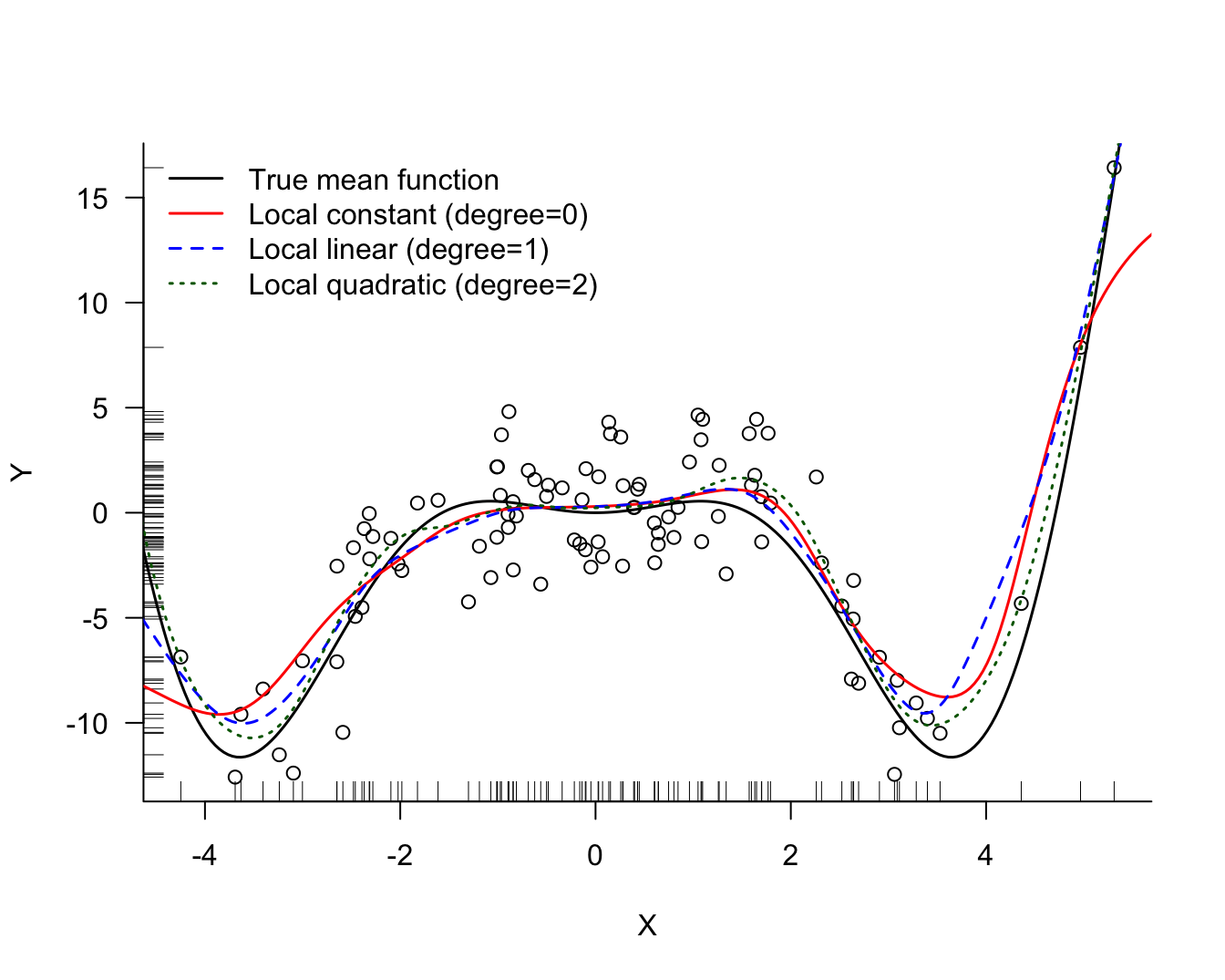
range.x =c(-5,6))The local quadratic model is the most flexible at the same bandwidth (Figure 11.7). All three estimates are similar in the interior of the \(x\) range. The boundary bias of the linear and quadratic model is much reduced compared to the kernel regression (degree 0) estimate.
For local polynomials of zero and first degree, the KernelReg function can be used. Specify reg_type='lc' for degree zero (local constant) and reg_type='ll' for degree one (local linear). For local polynomials of second degree and higher a different approach must be taken. One could use the KernelRidge function from sklearn with a second degree polynomial mean function and set the ridge parameter to a very small value, essentially turning off the ridge regularization.
import numpy as np
import statsmodels.api as sm
from statsmodels.nonparametric.kernel_regression import KernelReg
X = np.array(simReg.X).flatten()
Y = np.array(simReg.Y).flatten()
xGrid = np.linspace(-5, 6, 250)
xGrid = np.array(xGrid).flatten()
lp_05_0_model = KernelReg(endog=Y,exog=X,var_type='c',bw=[0.5],
reg_type='lc', # local constant (degree = 0)
)
lp_05_0_y, _ = lp_05_0_model.fit(xGrid)
# For degree = 1 (local linear regression)
lp_05_1_model = KernelReg(endog=Y,exog=X,var_type='c',bw=[0.5],
reg_type='ll', # local linear (degree = 1)
)
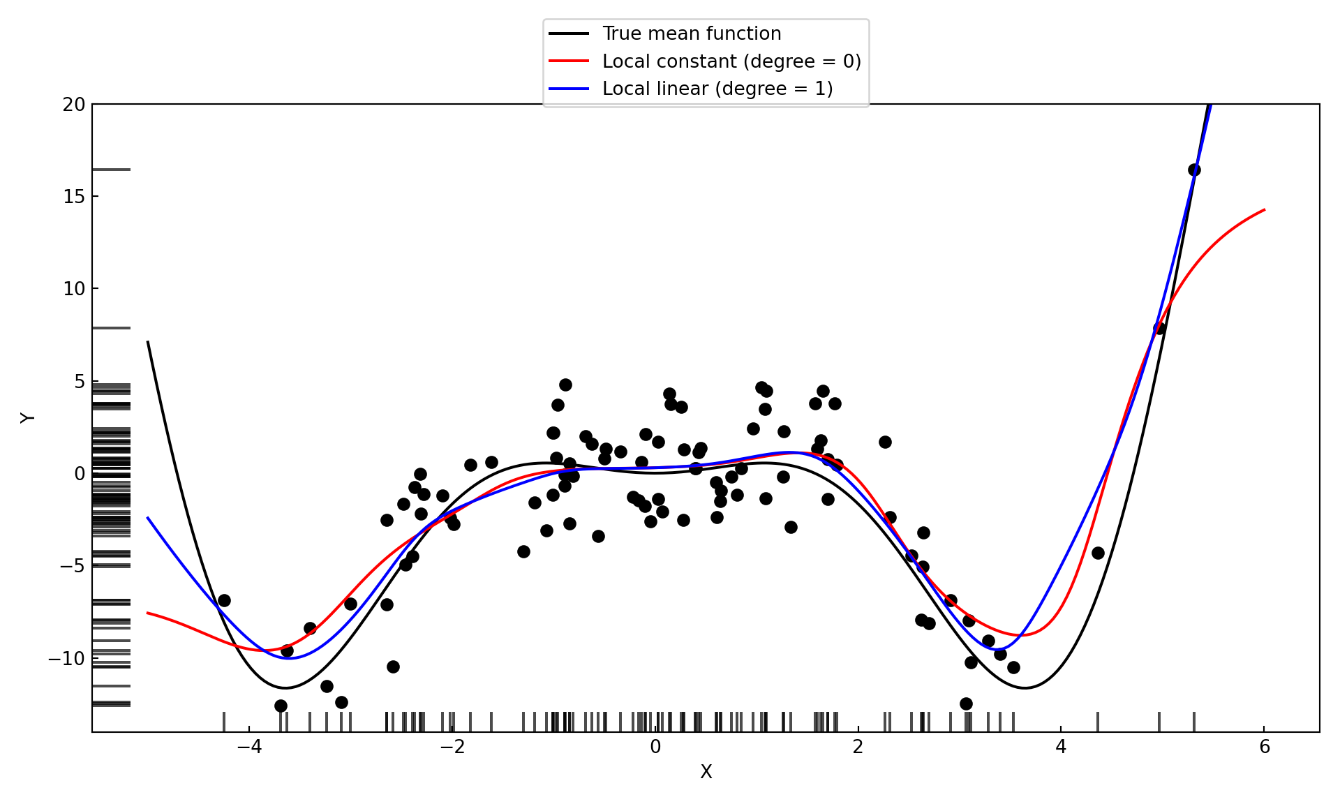
lp_05_1_y, _ = lp_05_1_model.fit(xGrid)The local linear model is more flexible at the same bandwidth than the local constant model. (Figure 11.8). The estimates are similar in the interior of the \(x\) range. The boundary bias of the linear model is much reduced compared to the kernel regression (degree 0) estimate.
Loess Regression
Loess (or LOESS) is a special case of local polynomial regression described by Cleveland (1979). The abbreviation stands for Local Estimated Scatterplot Smoothing. In terms of concepts introduced so far, Cleveland recommended a local linear model (degree 1) with a tricube kernel weight function and leave-one-out cross-validation to determine the bandwidth.
The tricube kernel was preferred because it reduces to exactly 0 and thus excludes observations outside of the tricube window from the calculations. The resulting computational savings were important at the time LOESS was proposed.
Example: LOESS Model of Degree 1 with Simulated Data
The loess function in R implements LOESS and specifies the bandwidth through a span parameter that determines the neighborhood of \(x_0\) as a proportion of the data points. The tricube weight function is then applied to the points in the spanned neighborhood. By default loess fits quadratic models with span=0.75. This value is fairly large for applications where you want to model \(Y\) as a function of \(X\), but works well in situations where you want to detect the presence of larger trends, as in the analysis of residuals.
Fitting of LOESS models and cross-validating the span parameter can be done conveniently in R with the train function in the caret package.
library(caret)

model <- caret::train(Y ~ X,
               data     =simReg,
               method   ="gamLoess",
               tuneGrid =expand.grid(span=0.2, degree=1),
               trControl=trainControl(method = "none"))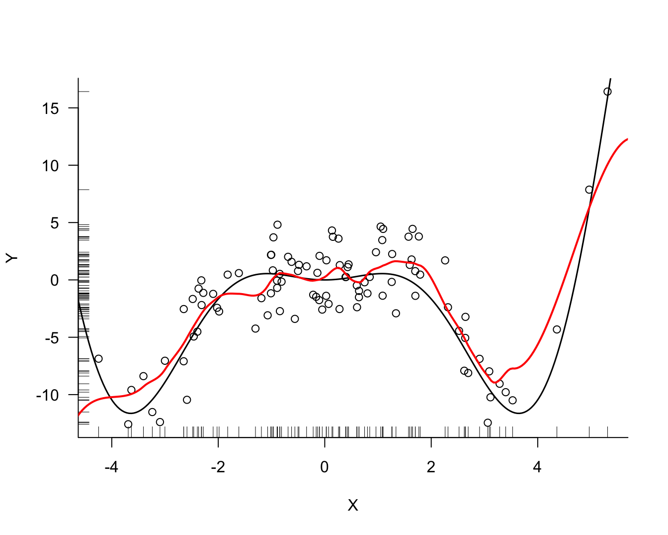
To perform cross-validation for the span parameter, you can supply instructions to the train function. The tuneGrid parameter provides a data frame with values for the hyperparameters. In the code below, the span is varied from 0.15 to 0.75 in 40 steps and the degree of the local polynomial is held fixed at 1. The trControl parameter defines the behavior of the train function. Here, 10-fold cross-validation of the hyperparameters is requested.
set.seed(3678)

ctrl <- trainControl(method="cv", number=10)
grid <- expand.grid(span=seq(0.15, 0.75, len=40), degree=1)

model <- train(Y ~ X,
               data     =simReg,
               method   ="gamLoess",
               tuneGrid =grid,
               trControl=ctrl)

print(model)
Generalized Additive Model using LOESS
100 samples
1 predictor
No pre-processing
Resampling: Cross-Validated (10 fold)
Summary of sample sizes: 89, 89, 90, 92, 91, 90, ...
Resampling results across tuning parameters:
span RMSE Rsquared MAE
0.1500000 2.901927 0.7325910 2.145192
0.1653846 2.919378 0.7336561 2.140403
0.1807692 2.615121 0.7373488 2.036346
0.1961538 2.624746 0.7364527 2.030095
0.2115385 2.656667 0.7304098 2.042989
0.2269231 2.668584 0.7263728 2.058201
0.2423077 2.679732 0.7206956 2.064964
0.2576923 2.694870 0.7175513 2.077081
0.2730769 2.757301 0.7032400 2.107686
0.2884615 2.787906 0.6907119 2.117425
0.3038462 2.811633 0.6848968 2.142258
0.3192308 2.831422 0.6761193 2.170968
0.3346154 2.885184 0.6611100 2.218675
0.3500000 2.967564 0.6400800 2.275226
0.3653846 3.004447 0.6280659 2.305204
0.3807692 3.066032 0.6113772 2.340453
0.3961538 3.097985 0.6022572 2.362501
0.4115385 3.163806 0.5835644 2.402466
0.4269231 3.203701 0.5713253 2.422956
0.4423077 3.257056 0.5567435 2.457546
0.4576923 3.292731 0.5471882 2.476899
0.4730769 3.338219 0.5342448 2.504264
0.4884615 3.351780 0.5291961 2.515220
0.5038462 3.391540 0.5169620 2.539841
0.5192308 3.443358 0.5013535 2.572879
0.5346154 3.478873 0.4891299 2.597151
0.5500000 3.501811 0.4799188 2.620423
0.5653846 3.536125 0.4668376 2.645889
0.5807692 3.592910 0.4487972 2.679671
0.5961538 3.645415 0.4337016 2.712018
0.6115385 3.605952 0.4463734 2.686381
0.6269231 3.574397 0.4561588 2.666609
0.6423077 3.623664 0.4421608 2.695329
0.6576923 3.605723 0.4552149 2.666462
0.6730769 3.632124 0.4461638 2.684623
0.6884615 3.650800 0.4401234 2.699304
0.7038462 3.667380 0.4341022 2.713919
0.7192308 3.690093 0.4270565 2.732718
0.7346154 3.710603 0.4196154 2.752871
0.7500000 3.743538 0.4038491 2.785017
Tuning parameter 'degree' was held constant at a value of 1
RMSE was used to select the optimal model using the smallest value.
The final values used for the model were span = 0.1807692 and degree = 1.plot(model)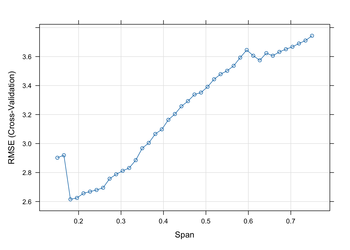
min(model$results$RMSE)[1] 2.615121model$results$span[which.min(model$results$RMSE)][1] 0.1807692The smallest root mean square error (RMSE) of 2.6151 is achieved with a span of 0.1808.
To fit a LOESS model of first degree in Python we can use the KernelReg function again, choosing the tricube kernel instead of the default Gaussian kernel and requesting reg_type='ll'.
from statsmodels.nonparametric.kernel_regression import KernelReg
X = np.array(simReg.X).flatten()
Y = np.array(simReg.Y).flatten()
xGrid = np.linspace(-5, 6, 250)
xGrid = np.array(xGrid).flatten()
loess_model = KernelReg(endog=Y, exog=X, var_type='c', ckertype='tricube',
reg_type='ll',
bw='cv_ls')
loess_mean, _ = kr_model.fit(xGrid)
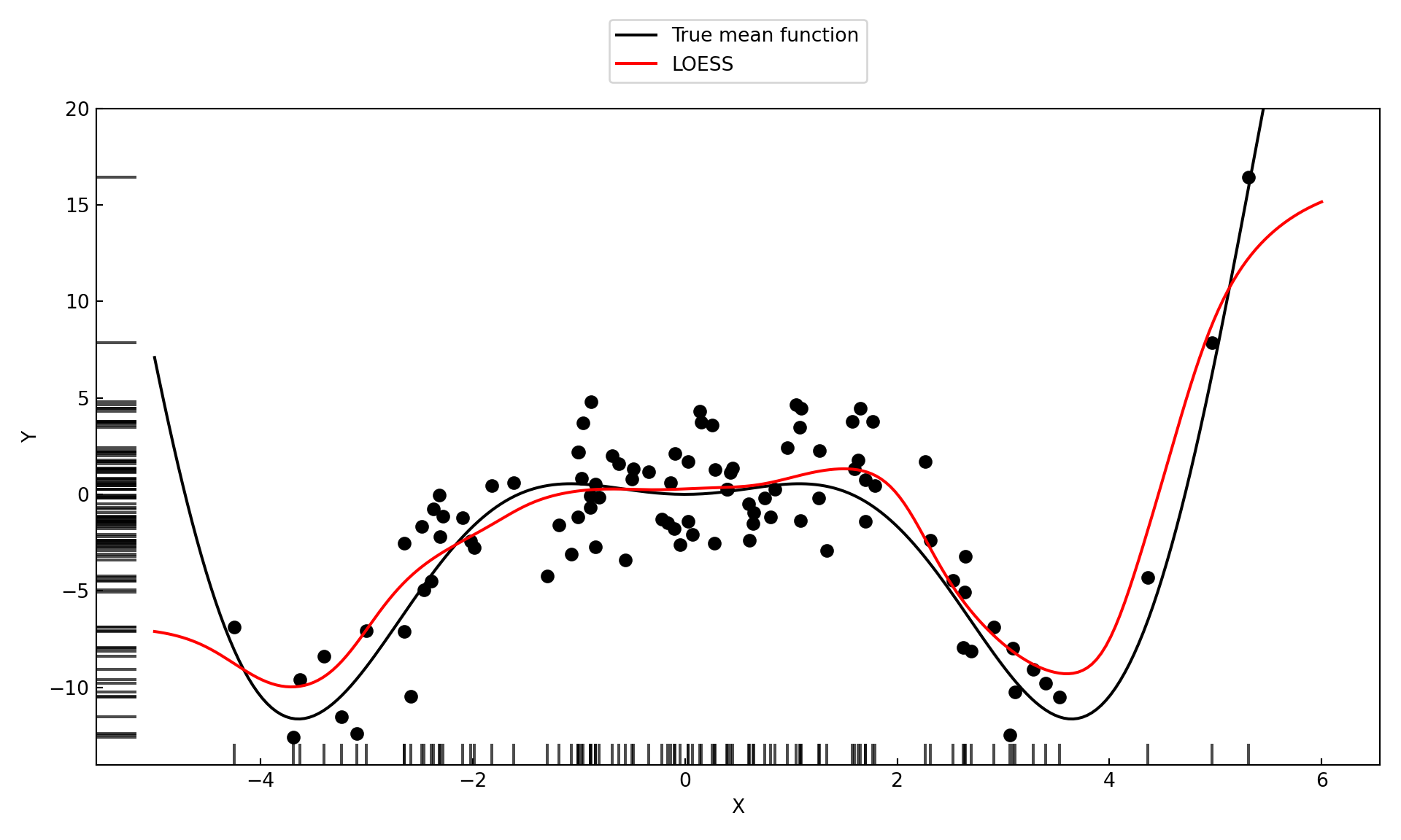
print(f"Cross-validated LOESS bandwidth: {loess_model.bw[0]:.4f}")Cross-validated LOESS bandwidth: 1.2140Figure 11.10 shows the fit of the LOESS model with the optimal bandwidth of 1.124.
11.3 Basis Functions
Segments, Knots, and Constraints
Local models using weight functions provide a lot of flexibility to model smooth functions based on a simple idea: if a constant, linear, or quadratic model approximates the local behavior at \(x_0\), then we can estimate the parameters of that local model through a weighted analysis that assigns weights to observations based on their distance from \(x_0\). Data points that are far from \(x_0\) will not have much impact on determining the local behavior if we choose the bandwidth of the kernel weight function properly.
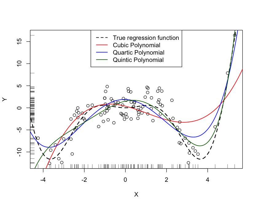
Greater flexibility in the fitted model could also be achieved by adding higher-order polynomial terms and fitting a global model. Unfortunately, this does not work well. Adding a higher-order term such as a cubic (\(x^3\)), quartic (\(x^4\)), or quintic (\(x^5\)) term to pick up curvature in one region can introduce strange behavior in another region. Figure 11.11 shows the fit of global polynomial models with up to third, fourth, and fifth degree terms for the simulated data. The quartic model \[ Y = \beta_0 + \beta_1x + \beta_2x^2 + \beta_3x^3 + \beta_4 x^4 + \epsilon \] does a pretty good job in capturing the curvature in the center of the \(x\) range. It could benefit from more flexibility in the upper region of \(x\), though. Adding a quintic term \(\beta_5 x^5\) to the model improves the fit for larger values of \(x\) but leads to poor behavior for small values of \(x\).
Can we introduce flexibility into the model by creating local behavior and avoid the uncontrolled behavior of higher-degree polynomials? The answer is “yes”, and splines is the way we achieve that.
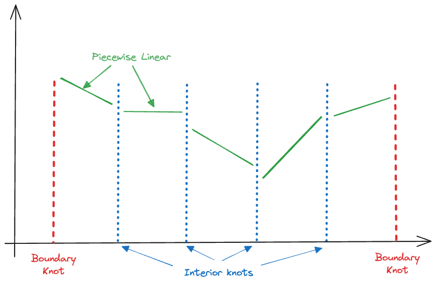
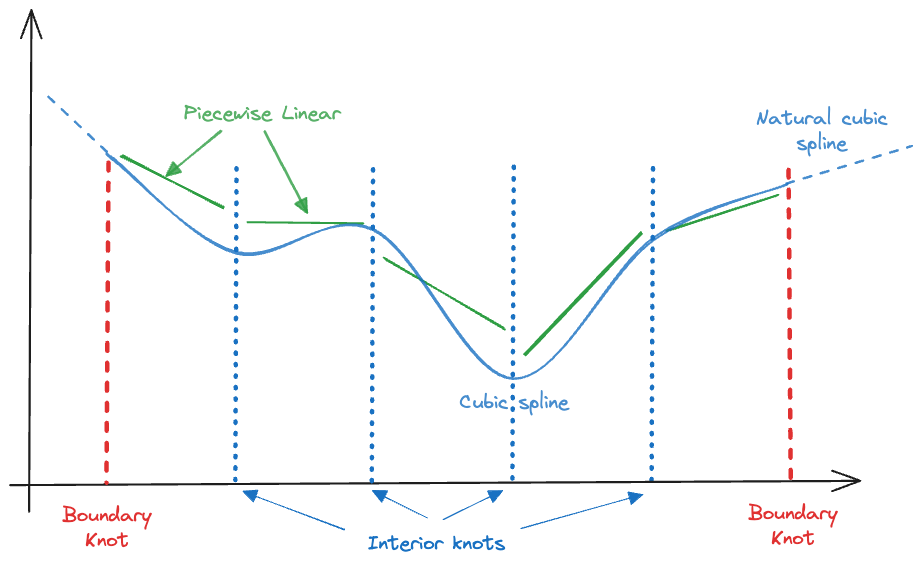
A spline model is a piecewise polynomial model. Rather than fitting a local model at every prediction point, a spline model connects polynomial models at specific points along the \(x\)-axis, called knots. As with global models, fitting a spline model and making predictions are separate steps. The model is local in the sense that we have different polynomials in different sections of the \(x\) range. Figure 11.12 displays the concept for piecewise polynomials of degree 1–that is, piecewise linear models. The extreme points of the \(x\) range serve as the boundary knots, four interior knots are evenly spaced along the \(x\) axis. This results in five linear segments. If we denote the interior knots as \(c_1, \cdots, c_4\), this piecewise linear model can be written as follows
\[ Y = \left \{ \begin{array}{ll} \beta_{01} + \beta_{11} x & x \le c_1 \\ \beta_{02} + \beta_{12}x & c_1 < x \le c_2 \\ \beta_{03} + \beta_{13}x & c_2 < x \le c_3 \\ \beta_{04} + \beta_{14}x & c_3 < x \le c_4 \\ \beta_{05} + \beta_{15}x & x > c_4 \\ \end{array} \right . \]
Each segment has a separate intercept and slope estimate. As the number of knots increases, the model becomes more localized and has more parameters.
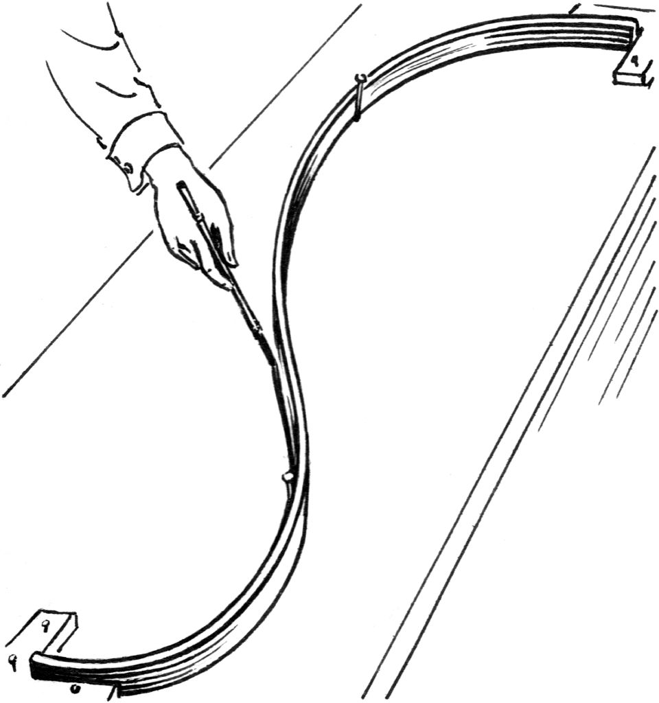
The name spline originates in construction where thin strips of wood were used to create curved shapes, for example, in shipbuilding. The strips of wood, called splines, are fixed at two points with devices called “dogs” or “ducks” and can be flexed between them (Figure 11.13).
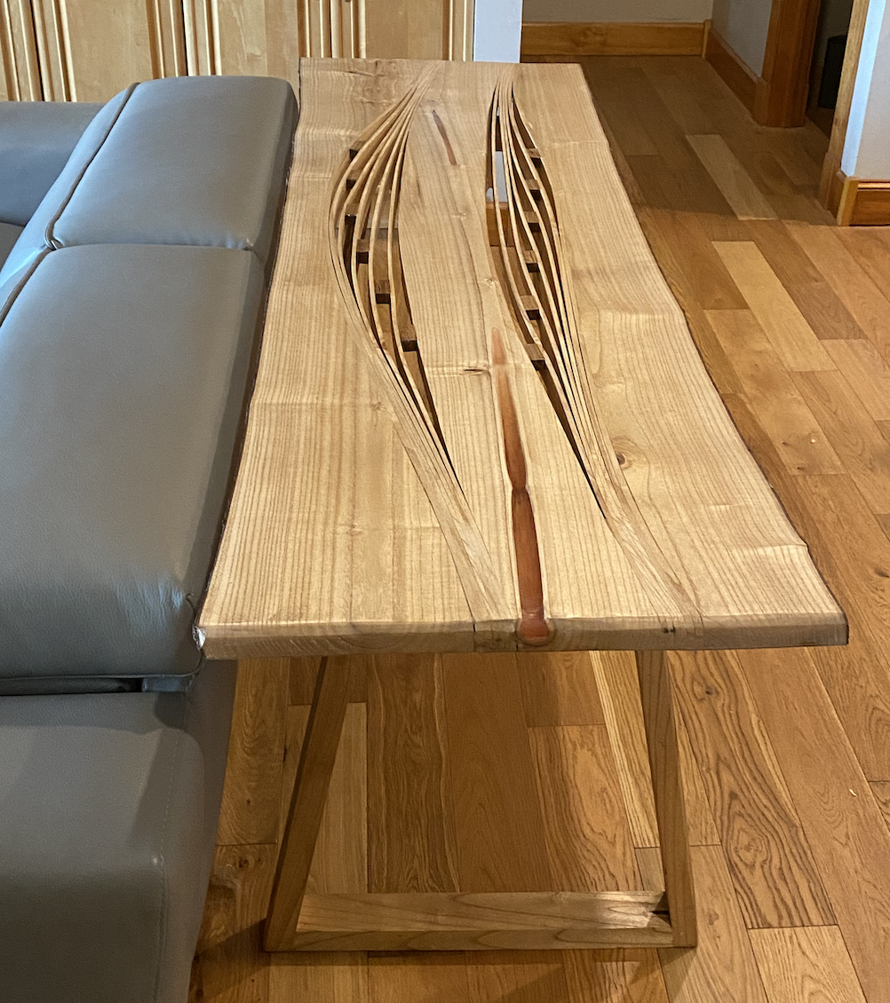
Spline Table
And now for something completely different! Inspired by the idea of a spline as a strip of wood bent around anchors, I built a table from Pauwlonia wood harvested and dried on my property in Blacksburg, VA. The splines are 3/8 inches thick strips of wood, flexed around small pieces of walnut. The legs are made from the same tree. The board milled from the center of the trunk was used for the curved piece in the middle of the table; its natural pith channel is filled with colored epoxy.
The segments in Figure 11.12 are not curved, that can be fixed by increasing the degree of the polynomial in each segment. But we recognize another problem with the piecewise linear model, the fitted lines do not connect at the segments. In order for the model to be continuous across the interior knots, the parameter estimates cannot be chosen freely–they have to obey certain constraints. For example, in order for the first two segments in Figure 11.12 to connect, we need to have \[ \beta_{01} + \beta_{11} c_1 = \beta_{02} + \beta_{12} c_1 \]
We would not be satisfied with the segments just touching at the knots, we also would want the spline to transition smoothly through the knots. So we can impose additional constraints on the polynomials. To ensure that the segments have the same slope at the knot we constrain their first derivative \[ \beta_{11} = \beta_{12} \]
With each constraint the number of free parameters in the model is reduced. We started with ten parameters in the model with four (interior) knots and disconnected lines (Figure 11.12). Imposing continuity at each knot imposes one constraint at each knot, leaving us with 6 free parameters (we are using 6 degrees of freedom for the model). Imposing continuity in the first derivative at each knot removes another 4 parameters, leaving us with 2 degrees of freedom. Without increasing the degree of the polynomial we will not be able to add further constraints. In fact, the continuous piecewise linear model with continuity in the first derivatives is just a global simple linear regression model.
To leave degrees of freedom to pick up local trends in the mean function we use cubic splines that are continuous at the knots and have the same first and second derivatives to be equal at the knots. A spline that satisfies those conditions is known as a cubic spline (Figure 11.14) or a degree-3 spline.
A spline of degree \(d\) in general is a piecewise polynomial of degree \(d\) with continuity constraints in the derivatives up to degree \(d-1\) at each knot. There is typically no need to engage splines of higher orders than cubic splines. They still have a discontinuity at the knots since they are continuous only up to second derivatives but it is said that the discontinuity is not visible to the human eye (Hastie, Tibshirani, and Friedman 2001, 134).
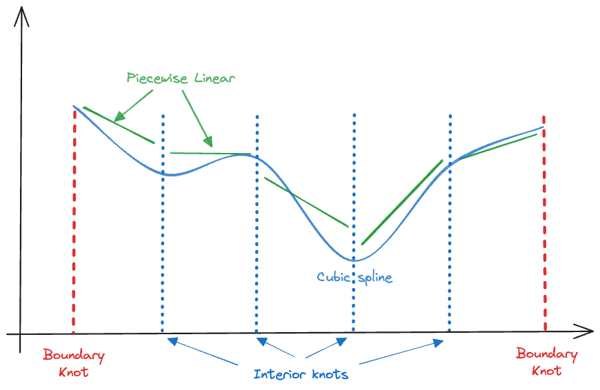
We also want to handle the boundary properly and are imposing another constraint: the model should have degree 1 beyond the range of \(x\) in the training data. This is known as a natural cubic spline (Figure 11.15). The natural cubic spline achieves linearity at the boundary by imposing additional constraints, two at each boundary knot. The four degrees of freedom made available–compared to the cubic spline–can be used to place an additional interior knot.
More degrees of freedom in the spline translates into more free parameters and more flexibility in the fit. For a cubic spline with \(K\) knots, there are \(K+1\) degree-3 polynomial segments that obey \(K\times 3\) constraints at the knots. The model thus uses \(4(K+1) - 3K = K+4\) degrees of freedom. The flexibility of a spline model increases with the number of knots.
Basis Function Representation
Fitting a spline model is a constrained optimization problem: minimize the residual sum of squares of the piecewise polynomial subject to the continuity constraints imposed on the parameters. There is a more direct way in which the model is written in a way that incorporates the constraints and a standard least-squares routine for linear models can be used.
Let’s think of our model in a slightly different formulation, \[ Y = \beta_0 + \beta_1 h_1(x) + \beta_2 h_2(x) + \cdots + \beta_p h_p(x) + \epsilon \] The functions \(h_1(x), \cdots, h_p(x)\) are known transformations of \(x\). For example, a third-degree polynomial has \(h_1(x)=x\), \(h_2(x)=x^2\), and \(h_3(x)=x^3\).
This is called the basis function representation of the linear model. The cubic spline model can be written as a third-degree polynomial augmented by truncated power basis functions. A truncated power basis function takes the general form
\[ t^n_+ = \left \{ \begin{array}{cc} t^n & t > 0 \\ 0 & t \le 0\end{array}\right . \]
The cubic spline model with \(K\) (interior) knots, written in terms of truncated power basis functions becomes \[ Y = \beta_0 + \beta_1 x + \beta_2 x^2 + \beta_3 x^3 + \beta_{3+1}(x-c_1)^3_+ + \cdots + \beta_{3+K}(x-c_K)^3_+ + \epsilon \tag{11.1}\]
For each knot, an input variable is added, its values are the 3-rd order truncated power basis functions of the distance from the \(k\)th knot. The model has \(K+4\) parameters, as expected for a cubic spline.
Example: Cubic Spline with 3 Knots
For the simulated data we can fit a cubic spline with 3 knots by constructing a model matrix for Equation 11.1 and passing it to a linear regression function. First we need to decide on the placement of the three knots. One option is to place knots evenly throughout the range of \(x\). Or, we can place knots at certain percentiles of the distribution of the \(x\) data. We choose the 1st, 2nd (median), and 3rd quartile here.
s <- summary(simReg$X)
c_1 <- s[2] # 1st. quartile
c_2 <- s[3] # median
c_3 <- s[5] # 3rd quartile

c_1
1st Qu.
-1.025803 c_2 Median
0.05192918 c_33rd Qu.
1.39678 tpf <- function(x,knot,degree) {
t <- ifelse(x > knot, (x-knot)^degree, 0)
}
X <- as.vector(simReg$X)
Xmatrix <- cbind(rep(1,length(X)), X, X^2, X^3,
tpf(X,c_1,3), tpf(X,c_2,3), tpf(X,c_3,3))
colnames(Xmatrix) <- c("Inctpt","x","x^2","x^3","tpf_c1","tpf_c2","tpf_c3")
round(Xmatrix[1:10,],4) Inctpt x x^2 x^3 tpf_c1 tpf_c2 tpf_c3
[1,] 1 0.4479 0.2006 0.0898 3.2003 0.0621 0.0000
[2,] 1 -2.3124 5.3474 -12.3656 0.0000 0.0000 0.0000
[3,] 1 0.8448 0.7137 0.6030 6.5459 0.4985 0.0000
[4,] 1 -2.6495 7.0199 -18.5993 0.0000 0.0000 0.0000
[5,] 1 0.2822 0.0796 0.0225 2.2377 0.0122 0.0000
[6,] 1 -1.0721 1.1494 -1.2323 0.0000 0.0000 0.0000
[7,] 1 -0.6232 0.3884 -0.2421 0.0653 0.0000 0.0000
[8,] 1 3.1122 9.6859 30.1447 70.8563 28.6608 5.0481
[9,] 1 -0.8961 0.8029 -0.7195 0.0022 0.0000 0.0000
[10,] 1 0.6422 0.4125 0.2649 4.6412 0.2057 0.0000Observations to the left of \(c_1\) = -1.0258 do not receive a contribution from the augmented power function terms, for example the second observation. Observation #8, which falls to the right of \(c_3\) = 1.3968 receives a contribution from all three truncated power function terms.
Now we pass the \(\textbf{X}\) matrix and \(\textbf{Y}\) vector to the lm.fit function to get the ordinary least squares coefficient estimates:
cub_spline <- lm.fit(x=Xmatrix,y=simReg$Y)
cub_spline$coefficients
Inctpt x x^2 x^3 tpf_c1 tpf_c2 tpf_c3
-4.324405 -11.263153 -6.970494 -0.951829 3.572409 -5.185659 4.441695 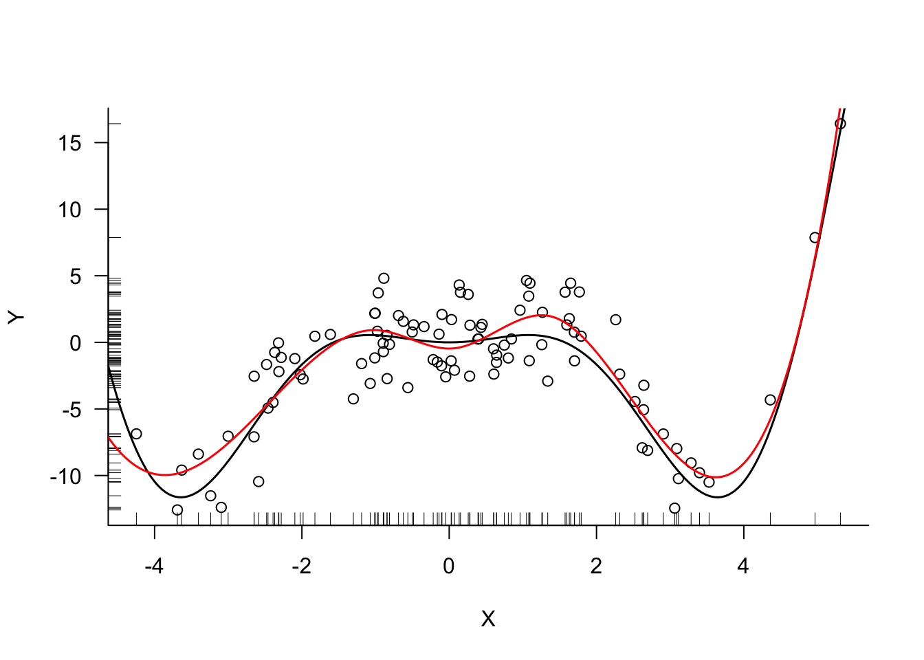
For a model with only seven parameters the cubic spline with knots at the 1st, 2nd, and 3rd quartile provides an excellent fit (Figure 11.16).
import numpy as np
import pandas as pd

s = np.percentile(simReg['X'], [25, 50, 75])
c_1 = s[0]  # 1st quartile
c_2 = s[1]  # median
c_3 = s[2]  # 3rd quartile

print(np.round(c_1,4))-1.0258print(np.round(c_2,4))0.0519print(np.round(c_3,4))1.3968# Define the truncated power function
def tpf(x, knot, degree):
return np.where(x > knot, (x - knot)**degree, 0)
# Create the design matrix
X = simReg['X'].values
ones = np.ones(len(X))
X_squared = X**2
X_cubed = X**3
tpf_c1 = tpf(X, c_1, 3)
tpf_c2 = tpf(X, c_2, 3)
tpf_c3 = tpf(X, c_3, 3)
Xmatrix = np.column_stack((ones, X, X_squared, X_cubed, tpf_c1, tpf_c2, tpf_c3))
Xmatrix_df = pd.DataFrame(Xmatrix,
columns=["Inctpt", "x", "x^2", "x^3", "tpf_c1", "tpf_c2", "tpf_c3"])
print(np.round(Xmatrix[:10], 4))[[ 1.00000e+00 4.47900e-01 2.00600e-01 8.98000e-02 3.20030e+00
6.21000e-02 0.00000e+00]
[ 1.00000e+00 -2.31240e+00 5.34740e+00 -1.23656e+01 0.00000e+00
0.00000e+00 0.00000e+00]
[ 1.00000e+00 8.44800e-01 7.13700e-01 6.03000e-01 6.54590e+00
4.98500e-01 0.00000e+00]
[ 1.00000e+00 -2.64950e+00 7.01990e+00 -1.85993e+01 0.00000e+00
0.00000e+00 0.00000e+00]
[ 1.00000e+00 2.82200e-01 7.96000e-02 2.25000e-02 2.23770e+00
1.22000e-02 0.00000e+00]
[ 1.00000e+00 -1.07210e+00 1.14940e+00 -1.23230e+00 0.00000e+00
0.00000e+00 0.00000e+00]
[ 1.00000e+00 -6.23200e-01 3.88400e-01 -2.42100e-01 6.53000e-02
0.00000e+00 0.00000e+00]
[ 1.00000e+00 3.11220e+00 9.68590e+00 3.01447e+01 7.08563e+01
2.86608e+01 5.04810e+00]
[ 1.00000e+00 -8.96100e-01 8.02900e-01 -7.19500e-01 2.20000e-03
0.00000e+00 0.00000e+00]
[ 1.00000e+00 6.42200e-01 4.12500e-01 2.64900e-01 4.64120e+00
2.05700e-01 0.00000e+00]]Observations to the left of \(c_1 = -1.0258\) do not receive a contribution from the augmented power function terms, for example the second observation. Observation #8, which falls to the right of \(c_3 = 1.3967\) receives a contribution from all three truncated power function terms.
Now we pass the \(\textbf{X}\) matrix and \(\textbf{Y}\) vector to the LinearReression function of sklearn to get the ordinary least squares coefficient estimates:
from sklearn.linear_model import LinearRegression

# Fit the model
model = LinearRegression(fit_intercept=False)
model.fit(Xmatrix, simReg['Y'])LinearRegression(fit_intercept=False)# Get coefficients
coefficients = model.coef_
print(np.round(coefficients,4))[ -4.3244 -11.2632 -6.9705 -0.9518 3.5724 -5.1857 4.4417](-14.032172932031724, 20.0)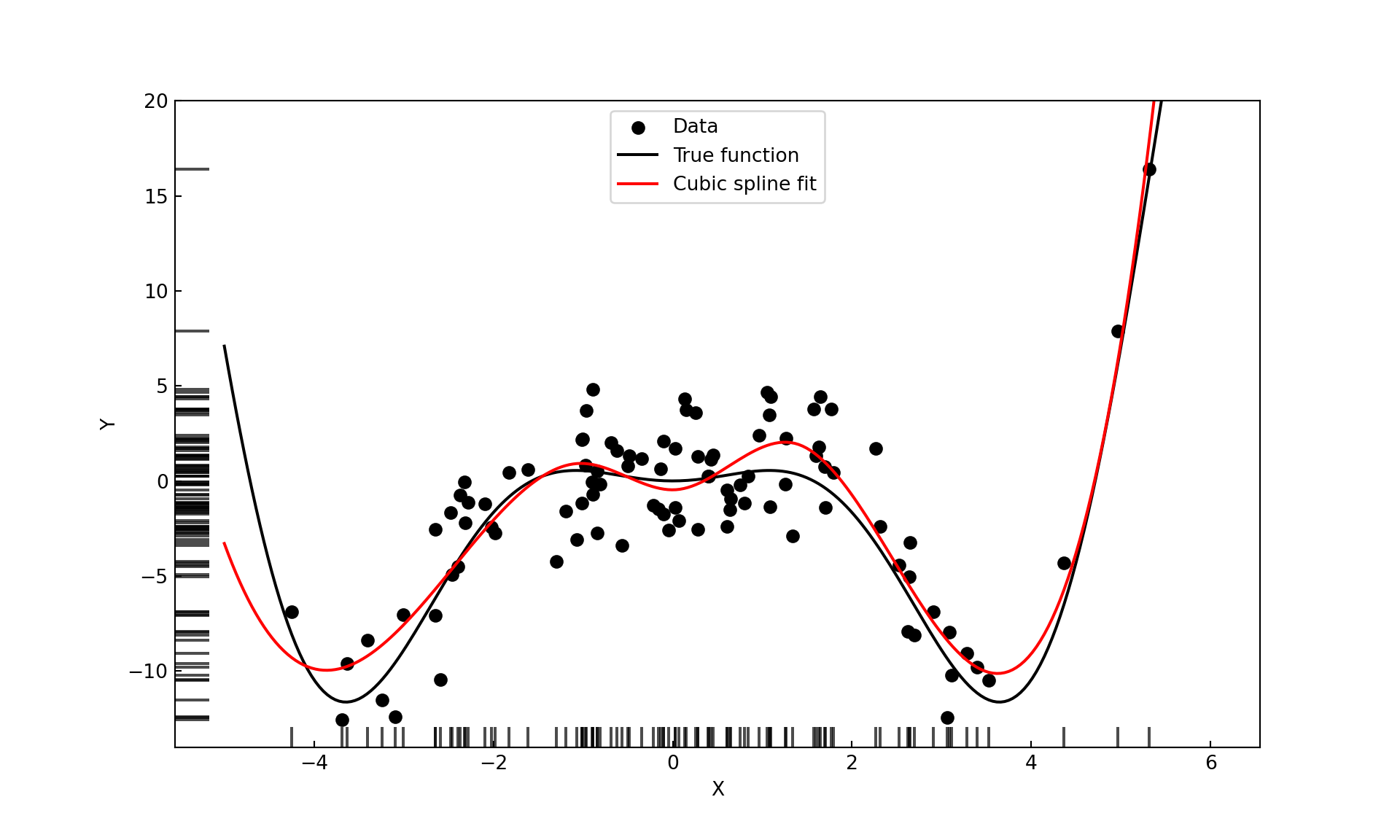
For a model with only seven parameters the cubic spline with knots at the 1st, 2nd, and 3rd quartile provides an excellent fit (Figure 11.17).
Regression Splines
The model in the previous example is known as a regression spline, characterized by placing a fixed number of knots. A common approach is to specify \(K\), the number of knots and placing knots at percentiles of the \(x\) values, as in the previous example. Another option is to place more knots in regions where the mean function is expected to vary more.
The truncated power basis function is one approach to generating the \(\textbf{X}\) matrix for a least-squares regression that produces a particular spline. It is not the numerically most advantageous approach. There are many equivalent basis functions to represent polynomials. A popular basis are the B-spline basis functions.
The R functions bs() and ns() in the splines library compute cubic spline matrices and natural cubic spline matrices based on B-splines.
library(splines)
xx <- bs(X,df=6)
attr(xx,"knots")
[1] -1.02580300 0.05192918 1.39678037The number of knots generated by bs() equals the chosen degrees of freedom minus the degree of the spline, which is 3 by default. The knots are placed at percentiles of \(x\), a third-order spline with 6 degrees of freedom results in 3 knots at the 1st, 2nd, and 3rd quartiles; the same values used earlier in the truncated power function example.
round(xx[1:10,],5) 1 2 3 4 5 6
[1,] 0.00000 0.04647 0.76826 0.18360 0.00167 0.00000
[2,] 0.40941 0.43423 0.09265 0.00000 0.00000 0.00000
[3,] 0.00000 0.00914 0.66063 0.31682 0.01340 0.00000
[4,] 0.47892 0.34084 0.05217 0.00000 0.00000 0.00000
[5,] 0.00000 0.07531 0.79106 0.13331 0.00033 0.00000
[6,] 0.07129 0.51921 0.40950 0.00000 0.00000 0.00000
[7,] 0.01545 0.38341 0.59720 0.00394 0.00000 0.00000
[8,] 0.00000 0.00000 0.08153 0.39302 0.44131 0.08414
[9,] 0.04277 0.47603 0.48107 0.00013 0.00000 0.00000
[10,] 0.00000 0.02336 0.72313 0.24798 0.00553 0.00000Although the xx matrix produced by bs() is not identical to the Xmatrix based on the truncated power basis functions, the models are equivalent and the predicted values are identical. The conditioning of the \(\textbf{X}^\prime\textbf{X}\) matrix based on the truncated power basis is poorer than the conditioning of the \(\textbf{X}^\prime\textbf{X}\) matrix computed from the B-spline basis. The pairwise correlations are generally higher in the former.
round(cor(Xmatrix[,2:7]),5) x x^2 x^3 tpf_c1 tpf_c2 tpf_c3
x 1.00000 0.20112 0.82204 0.71892 0.63024 0.50541
x^2 0.20112 1.00000 0.42635 0.76803 0.77741 0.73487
x^3 0.82204 0.42635 1.00000 0.89977 0.88997 0.84555
tpf_c1 0.71892 0.76803 0.89977 1.00000 0.98705 0.92475
tpf_c2 0.63024 0.77741 0.88997 0.98705 1.00000 0.97202
tpf_c3 0.50541 0.73487 0.84555 0.92475 0.97202 1.00000round(cor(xx),5) 1 2 3 4 5 6
1 1.00000 0.46034 -0.59238 -0.49291 -0.29365 -0.13162
2 0.46034 1.00000 -0.08910 -0.75758 -0.48386 -0.21712
3 -0.59238 -0.08910 1.00000 -0.00750 -0.45067 -0.30818
4 -0.49291 -0.75758 -0.00750 1.00000 0.59160 -0.05045
5 -0.29365 -0.48386 -0.45067 0.59160 1.00000 0.28366
6 -0.13162 -0.21712 -0.30818 -0.05045 0.28366 1.00000The function ns() produces the natural cubic splines from the B-spline basis.
nn <- ns(X,df=6)
round(nn[1:10,],5)
1 2 3 4 5 6
[1,] 0.01539 0.53224 0.44483 0.00664 0.00211 -0.00122
[2,] 0.24048 0.00000 0.00000 -0.20417 0.48178 -0.27761
[3,] 0.00000 0.24623 0.69323 0.05335 0.01697 -0.00978
[4,] 0.13541 0.00000 0.00000 -0.20501 0.48376 -0.27875
[5,] 0.04383 0.63577 0.31891 0.00131 0.00042 -0.00024
[6,] 0.68611 0.15236 0.00000 -0.05195 0.12258 -0.07063
[7,] 0.54971 0.41216 0.00251 -0.01149 0.02711 -0.01562
[8,] 0.00000 0.00000 0.13784 0.50699 0.26615 0.08901
[9,] 0.66500 0.23641 0.00000 -0.03179 0.07502 -0.04323
[10,] 0.00205 0.38855 0.58442 0.02201 0.00700 -0.00404The models can be fit without first generating the spline matrix:
ns_spline <- lm(simReg$Y ~ ns(X,df=6))
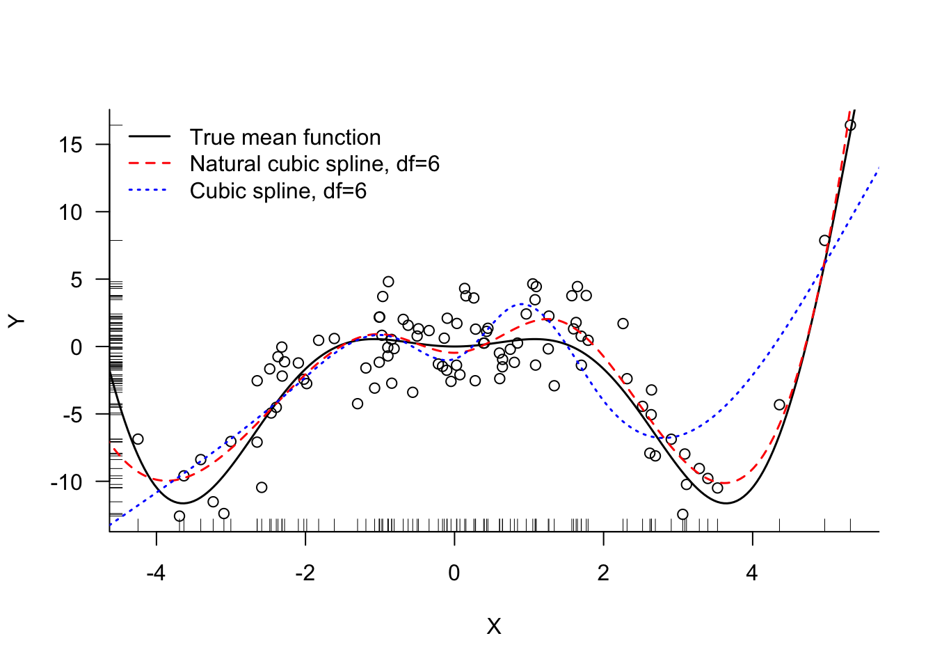
bs_spline <- lm(simReg$Y ~ bs(X,df=6))Figure 11.18 displays the fitted values for the 6-df cubic and natural cubic splines.
In Python you can compute B-splines and cubic regression splines using the dmatrix function in patsy. The bs() and cr() formula arguments of patsy represent those splines.
from patsy import dmatrix
from scipy.stats import pearsonr

# For natural and B-splines, we'll use patsy which provides similar functionality to R's splines
# Equivalent to bs(X, df=6) in R
xx = dmatrix("bs(x, df=6)", {"x": X}, return_type='dataframe')

print(xx.columns)
Index(['Intercept', 'bs(x, df=6)[0]', 'bs(x, df=6)[1]', 'bs(x, df=6)[2]',
'bs(x, df=6)[3]', 'bs(x, df=6)[4]', 'bs(x, df=6)[5]'],
dtype='object')# Print first 10 rows of the B-spline basis
np.set_printoptions(suppress=True)
print(np.round(xx.values[:10], 5))[[1. 0. 0.04647 0.76826 0.1836 0.00167 0. ]
[1. 0.40941 0.43423 0.09265 0. 0. 0. ]
[1. 0. 0.00914 0.66063 0.31682 0.0134 0. ]
[1. 0.47892 0.34084 0.05217 0. 0. 0. ]
[1. 0. 0.07531 0.79106 0.13331 0.00033 0. ]
[1. 0.07129 0.51921 0.4095 0. 0. 0. ]
[1. 0.01545 0.38341 0.5972 0.00394 0. 0. ]
[1. 0. 0. 0.08153 0.39302 0.44131 0.08414]
[1. 0.04277 0.47603 0.48107 0.00013 0. 0. ]
[1. 0. 0.02336 0.72313 0.24798 0.00553 0. ]]Although the xx matrix produced by bs() is not identical to the Xmatrix based on the truncated power basis functions, the models are equivalent and the predicted values are identical. The conditioning of the \(\textbf{X}^\prime\textbf{X}\) matrix based on the truncated power basis is poorer than the conditioning of the \(\textbf{X}^\prime\textbf{X}\) matrix computed from the B-spline basis. The pairwise correlations are generally higher in the former.
corr_mat = np.corrcoef(Xmatrix[:, 1:7], rowvar=False)
print(np.round(corr_mat, 5))
[[1. 0.20112 0.82204 0.71892 0.63024 0.50541]
[0.20112 1. 0.42635 0.76803 0.77741 0.73487]
[0.82204 0.42635 1. 0.89977 0.88997 0.84555]
[0.71892 0.76803 0.89977 1. 0.98705 0.92475]
[0.63024 0.77741 0.88997 0.98705 1. 0.97202]
[0.50541 0.73487 0.84555 0.92475 0.97202 1. ]]bs_corr = np.corrcoef(xx.values, rowvar=False)
print("Correlation of B-spline basis:")Correlation of B-spline basis:print(np.round(bs_corr[1:6,1:6], 5))[[ 1. 0.46034 -0.59238 -0.49291 -0.29365]
[ 0.46034 1. -0.0891 -0.75758 -0.48386]
[-0.59238 -0.0891 1. -0.0075 -0.45067]
[-0.49291 -0.75758 -0.0075 1. 0.5916 ]
[-0.29365 -0.48386 -0.45067 0.5916 1. ]]The cr() argument of dmatrix produces cubic regression splines. These match the implementation in the mgcv package in R, rather than the ns function.
nn = dmatrix("cr(x, df=6)", {"x": X}, return_type='dataframe')
print("First 10 rows of natural spline basis:")
First 10 rows of natural spline basis:print(np.round(nn.values[:10], 4))[[ 1. 0.0006 -0.0077 0.0524 0.9779 -0.024 0.0008]
[ 1. 0.0969 1.1184 -0.2998 0.0998 -0.0158 0.0006]
[ 1. -0.0019 0.0234 -0.1578 0.9276 0.2154 -0.0068]
[ 1. 0.2074 1.0775 -0.3967 0.132 -0.0209 0.0007]
[ 1. 0.0025 -0.0315 0.2239 0.8671 -0.0643 0.0023]
[ 1. -0.0254 0.3924 0.8072 -0.2057 0.0326 -0.0011]
[ 1. -0.005 0.0626 1.0231 -0.0953 0.0151 -0.0005]
[ 1. 0.0026 -0.0325 0.2187 -0.7718 1.3413 0.2417]
[ 1. -0.0178 0.2475 0.9363 -0.1959 0.0311 -0.0011]
[ 1. -0.001 0.0129 -0.0868 1.0076 0.0697 -0.0024]]We now fit the models based on the B-splines and cubic regression splines.
import statsmodels.api as sm

X_ns = dmatrix("cr(x, df=6)", {"x": X})
model_ns = sm.OLS(simReg['Y'], X_ns).fit()
#model_ns.summary()

X_bs = dmatrix("bs(x, df=6)", {"x": X})
model_bs = sm.OLS(simReg['Y'], X_bs).fit()
#model_bs.summary()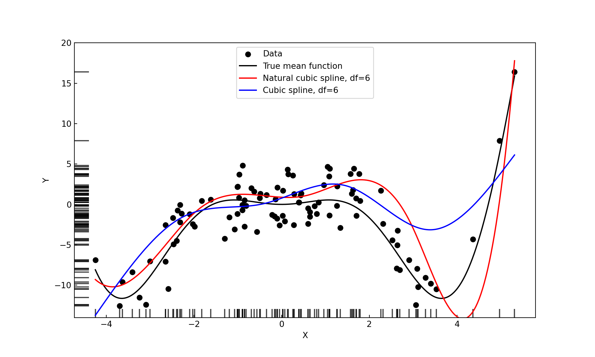
An objective method for choosing the number of knots in regression splines is through cross-validation.
Example: Choosing Degrees of Freedom by Cross-validation
The following code use the caret::train function in R to choose the degrees of freedom of the cubic spline based on 10-fold cross-validation. The degrees of freedom evaluated range from 2 to 20.
set.seed(3678)

ctrl <- trainControl(method = "cv", number = 10)
grid <- expand.grid(df = seq(2,20,by=1))

model <- train(Y ~ X,
               data     =simReg,
               method   ="gamSpline",
               tuneGrid =grid,
               trControl=ctrl)

model
Generalized Additive Model using Splines
100 samples
1 predictor
No pre-processing
Resampling: Cross-Validated (10 fold)
Summary of sample sizes: 89, 89, 90, 92, 91, 90, ...
Resampling results across tuning parameters:
df RMSE Rsquared MAE
2 4.044198 0.3076557 3.020568
3 3.659884 0.4245450 2.749611
4 3.304364 0.5299490 2.565251
5 2.989824 0.6241050 2.373329
6 2.749716 0.6861406 2.208537
7 2.589525 0.7207527 2.094446
8 2.489518 0.7400459 2.028971
9 2.427930 0.7516088 1.999040
10 2.389342 0.7591292 1.983502
11 2.364524 0.7643125 1.973074
12 2.348485 0.7679405 1.965031
13 2.338639 0.7703677 1.959352
14 2.333664 0.7717649 1.955700
15 2.332962 0.7722239 1.955451
16 2.336070 0.7718901 1.957769
17 2.343017 0.7708601 1.961188
18 2.353694 0.7692620 1.965484
19 2.368154 0.7672486 1.973497
20 2.386424 0.7648974 1.982863
RMSE was used to select the optimal model using the smallest value.
The final value used for the model was df = 15.plot(model)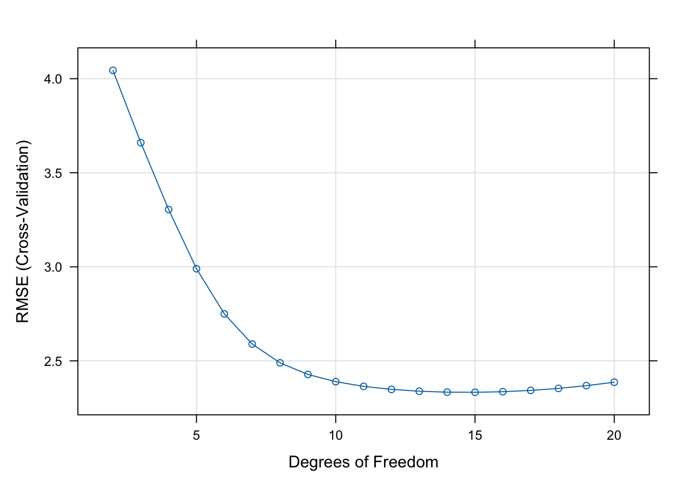
The square root of the mean square error (RMSE) achieves a minimum for df=15 although any value between 12 and 17 is reasonable.
Next, the final model is trained using the degrees of freedom chosen by cross-validation.
model <- train(Y ~ X,
               data     =simReg,
               method   ="gamSpline",
               tuneGrid =expand.grid(df=model$bestTune$df),
               trControl=trainControl(method = "none"))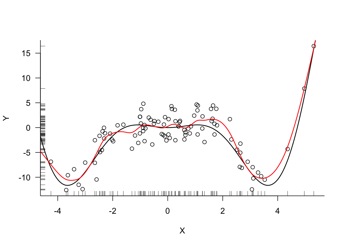
import numpy as np
import pandas as pd
import matplotlib.pyplot as plt
from patsy.builtins import bs, cr
import statsmodels.api as sm

# Define a function to evaluate models
def train_spline_model(X, y, param_grid):
    results = {'param': [], 'mean_test_score': []}

    for ddf in param_grid['ddf']:
        formula_str = f"bs(x, df={ddf}, include_intercept=True)"
        Xmat = dmatrix(formula_str, {"x": X})
        mlr = sm.OLS(y, Xmat).fit()
        leverage = mlr.get_influence().hat_matrix_diag
        PRESS_res = mlr.resid / (1 - leverage)
        PRESS = np.sum(PRESS_res**2)

        results['param'].append(ddf)
        results['mean_test_score'].append(PRESS/len(leverage))

    # Find best parameter
    best_idx = np.argmin(results['mean_test_score'])
    best_param = results['param'][best_idx]

    return results, best_param

param_grid = {'ddf': list(range(5, 25))}

# Train the model
X_array = simReg['X'].values
y_array = simReg['Y'].values
results, best_df = train_spline_model(X_array, y_array, param_grid)


# Print results
print(f"Best df parameter: {best_df}")
Best df parameter: 15print("Cross-validation results:")Cross-validation results:for i, df in enumerate(results['param']):
print(f"df: {df}, RMSE: {np.sqrt(results['mean_test_score'][i])}")df: 5, RMSE: 3.3494655985628214
df: 6, RMSE: 3.333430963099322
df: 7, RMSE: 2.5600955191315475
df: 8, RMSE: 2.4241591379424614
df: 9, RMSE: 2.48726729289632
df: 10, RMSE: 2.489860338881902
df: 11, RMSE: 2.4360366916977227
df: 12, RMSE: 2.592839044844069
df: 13, RMSE: 2.535736048682191
df: 14, RMSE: 2.3739688144209783
df: 15, RMSE: 2.349363259071974
df: 16, RMSE: 2.5471341829902148
df: 17, RMSE: 2.6489271113256283
df: 18, RMSE: 3.19081969490032
df: 19, RMSE: 4.045579899824276
df: 20, RMSE: 4.478177576623424
df: 21, RMSE: 4.851501067897742
df: 22, RMSE: 5.435138928463077
df: 23, RMSE: 5.911951785412853
df: 24, RMSE: 6.358454700512752# Plot the results
plt.figure(figsize=(10, 6));
plt.plot(results['param'], np.array(results['mean_test_score']));
plt.xlabel('Degrees of Freedom');
plt.ylabel('RMSE');
plt.title('Cross-Validation Results');
plt.grid(True);
plt.show();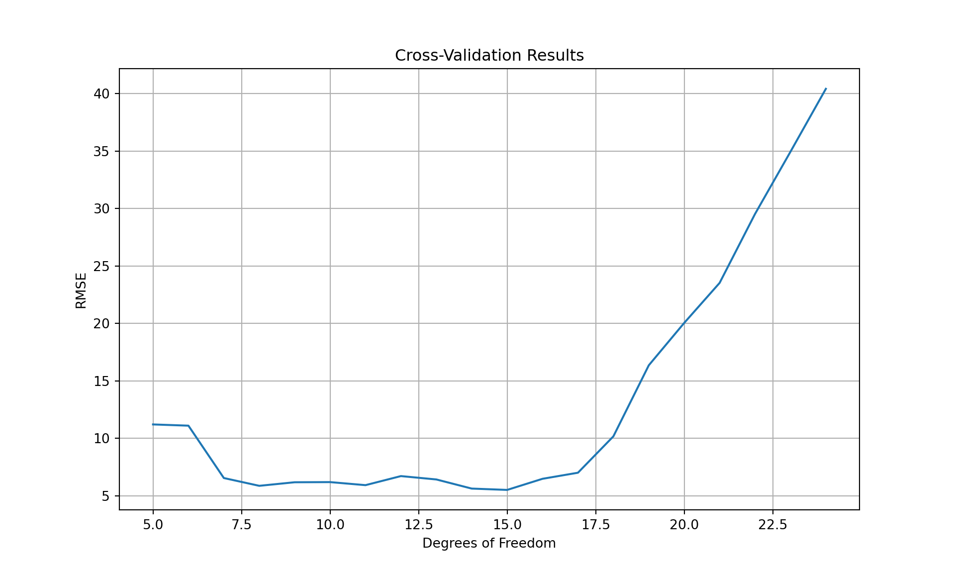
The square root of the mean square error (RMSE) achieves a minimum for 15 degrees of freedom although any value between 13 and 15 is reasonable.
Next, the final model is trained using the degrees of freedom chosen by cross-validation and predicted values are computed for a grid of \(X\)-values.
formula_str = f"bs(x, df={best_df})"
Xmat = dmatrix(formula_str, {"x": X_array})
mlr = sm.OLS(y_array, Xmat).fit()

XGrid_mat = dmatrix(formula_str, {"x": xGrid})
pred = mlr.predict(XGrid_mat)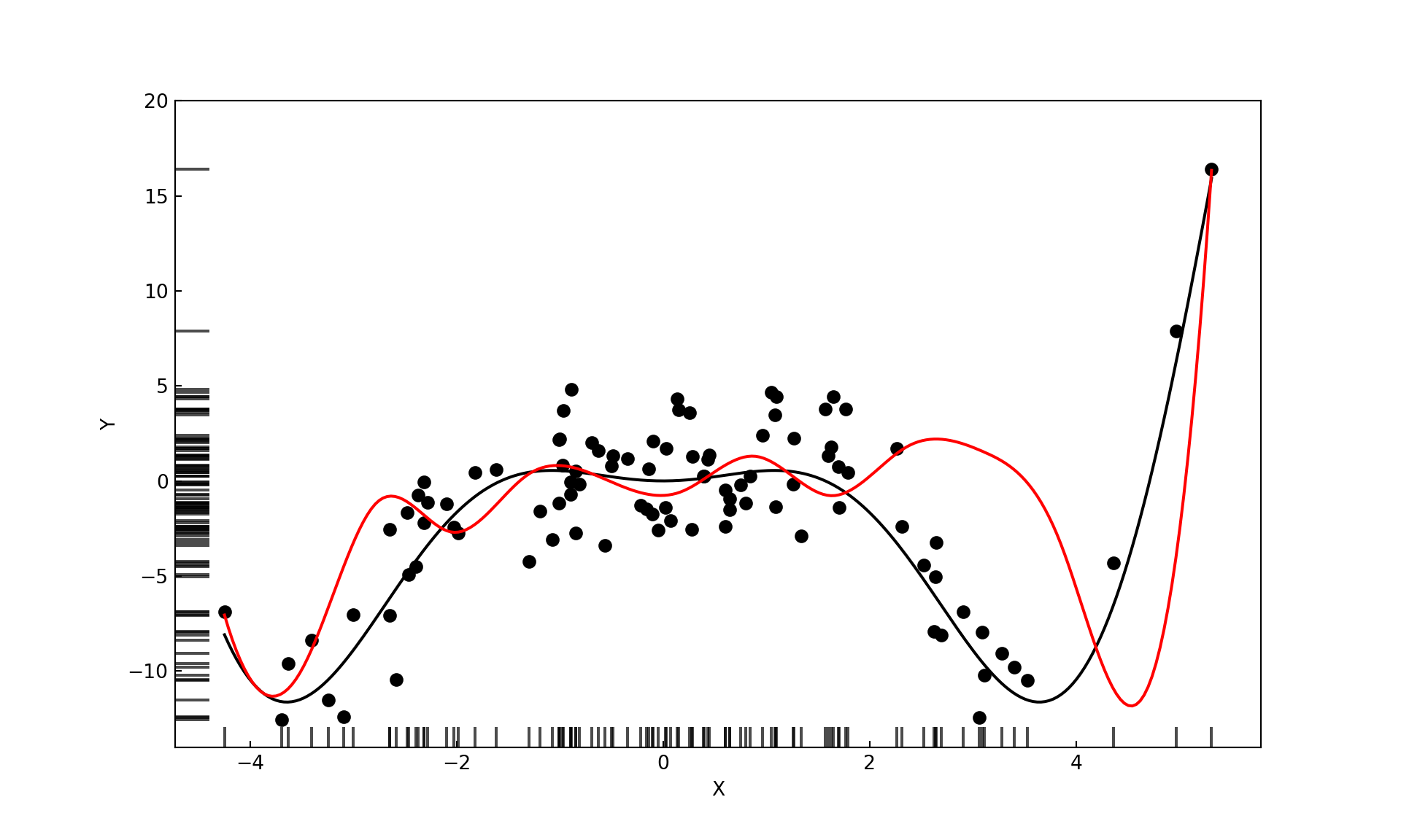
Smoothing Splines
Regression splines require specification of the number of knots \(K\) and their placement \(c_1, \cdots, c_K\). Equivalently, the degrees of freedom of the spline can be specified instead of \(K\). Choosing \(K\) too small results in bias and choosing \(K\) too large leads to overfit models with high variance.
Smoothing splines approach the issue of knot placement from a different angle. Why not place knots at all unique values of \(X\)? This creates a high-dimensional problem that can be adjusted through regularization. This resolves the questions of knot number and knot placement and shifts attention from cross-validating \(K\) to choosing the regularization parameter.
The regularization penalty for smoothing splines is \[ \lambda \int f^{\prime\prime}(v)\,dv \] where \(f^{\prime\prime}\) denotes the second derivative of the mean function and \(\lambda\) is the hyperparameter. The rationale for this penalty term is as follows: the second derivative \(f^{\prime\prime}(x)\) measures the curvature of \(f\) at \(x\). High absolute values indicate that \(f\) changes quickly in the neighborhood of \(x\), the sign of a wiggly function. The integral of the second derivative can be interpreted as the degree of wiggliness across the range of \(x\).
For a given value of \(\lambda\) more wiggly functions result in a higher penalty. For \(\lambda = 0\) no penalty is added. The basic model for a smoothing spline is a cubic spline with knots at all unique \(x\)-values. The regularization penalty shrinks the coefficient estimates of the spline and reduces the variability of the fitted function this way.
An interesting aspect are the effective or equivalent degrees of freedom. The smoothing spline has \(n\) parameters but these are shrunk if the penalty term kicks in. The equivalent degrees of freedom measure the flexibility of the fitted function. Mathematically, the fitted values of a smoothing spline is a linear function of the observed data. For each value \(\lambda\), the solution can be written as
\[ \widehat{y}_\lambda = \textbf{S}_\lambda \textbf{y} \] where \(\textbf{S}_\lambda\) is the smoother matrix, akin to the “Hat” matrix in global regression models. Recall from Section 3.6.2 that the Hat matrix is an orthogonal projection matrix and its trace equals the number of parameters (the degrees of freedom) of the model. Similarly, the equivalent degrees of freedom of a smoother are obtained as the trace of the smoother matrix, \[ df_\lambda = tr(\textbf{S}_\lambda) = \sum_{i=1}^n [s_{ii}]_\lambda \]
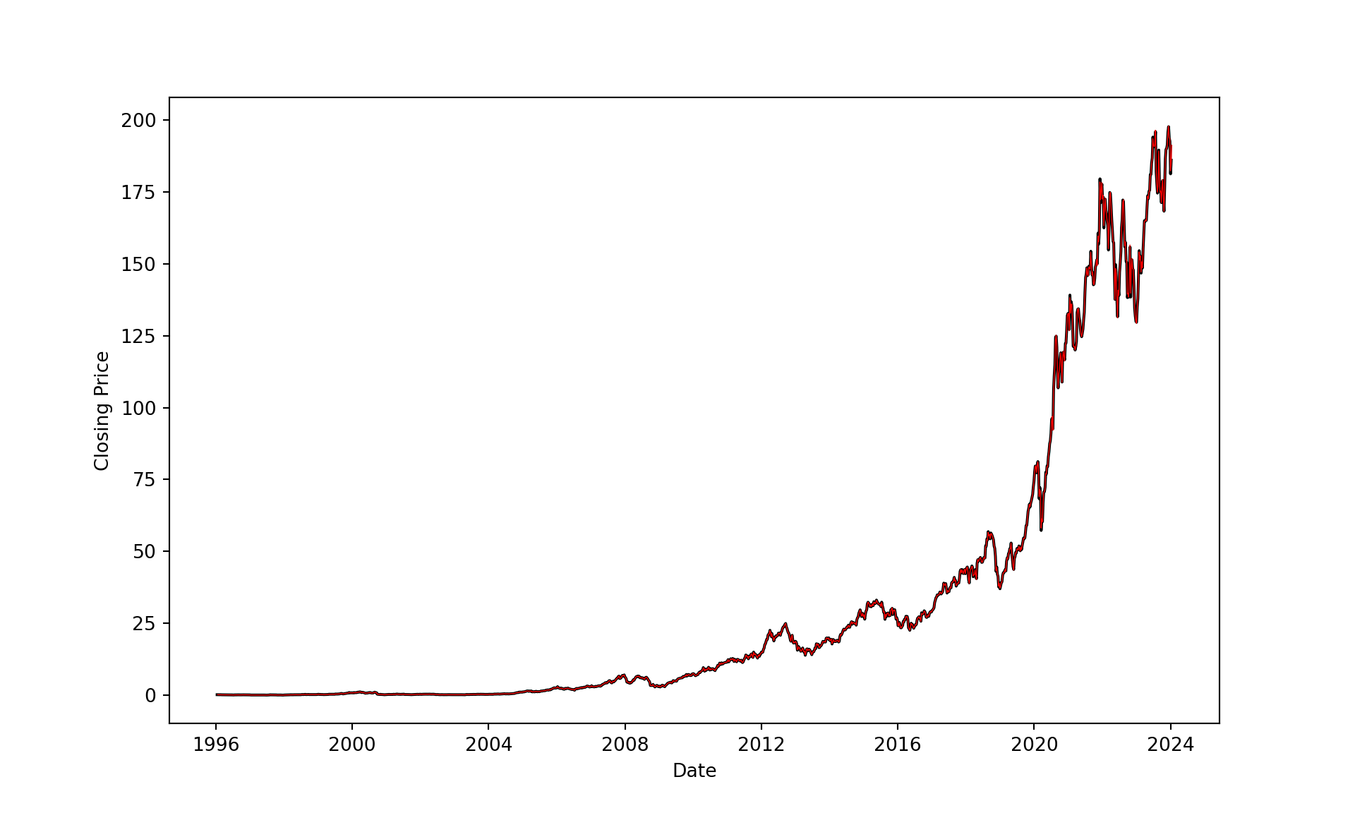
Example: Apple Share Prices
The data for this example are the weekly closing share prices of Apple (ticker symbol AAPL) between January 1996 and January 2024. Figure 11.20 shows a time series of these prices along with the dates major Apple products were introduced.
library(splines)
library(lubridate)
library("duckdb")

con <- dbConnect(duckdb(),dbdir = "ads.ddb",read_only=TRUE)
weekly <- dbGetQuery(con, "SELECT * FROM AAPLWeekly")
weekly$date <- make_date(weekly$year,weekly$month,weekly$day)

dbDisconnect(con)
import duckdb
import pandas as pd
from datetime import date
con = duckdb.connect(database="ads.ddb", read_only=True)
weekly = con.sql("SELECT * FROM AAPLWeekly;").df()
con.close()
weekly['date'] = pd.to_datetime({'year': weekly['year'],
'month': weekly['month'],
'day': weekly['day']})
#Alternatively, if you need a Python date object rather than pandas datetime:
#from datetime import date
#weekly['date'] = weekly.apply(lambda row: date(row['year'], row['month'], row['day']), axis=1)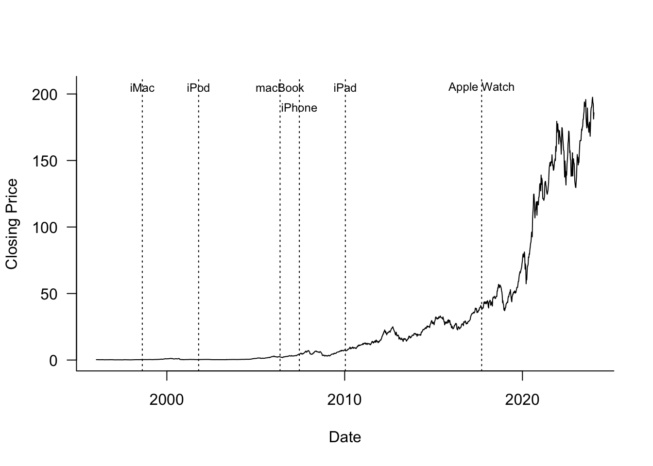
The smooth.spline function in R computes smoothing splines and selects the smoothing parameter (the penalty hyperparameter) by leave-one-out cross-validation. It should be noted that smooth.spline by default does not place knots at all unique \(x\) values, but places evenly-spaced knots, their number is a function of the unique number of \(x\)-values. You can change this behavior by setting all.knots=TRUE.
In the AAPL example, there are 1,461 unique dates, and smooth.spline would choose 154 knots by default.
# general method for computing the number of unique values in a numeric vector
nx <- length(weekly$date) -
      sum(duplicated(round((weekly$date - mean(weekly$date))/1e-6)))
nx
[1] 1461.nknots.smspl(nx)[1] 154smspl_a <- smooth.spline(y=weekly$Close,
x=weekly$date,
all.knots=TRUE,
cv=TRUE)
smspl_aCall:
smooth.spline(x = weekly$date, y = weekly$Close, cv = TRUE, all.knots = TRUE)
Smoothing Parameter spar= 0.3941696 lambda= 1.661548e-10 (11 iterations)
Equivalent Degrees of Freedom (Df): 607.3517
Penalized Criterion (RSS): 1235.319
PRESS(l.o.o. CV): 2.544907The cross-validation leads to a PRESS criterion of 2.5449 and equivalent degrees of freedom of 607.352. The regularization penalized the spline from 1461 interior knots to the equivalent of a spline with about 610 knots. The smoothing parameter spar has a substantial value of 0.3942.
Setting all.knots=FALSE leads to the following analysis
smspl_s <- smooth.spline(y=weekly$Close,
                         x=weekly$date,
                         all.knots=FALSE,
                         cv=TRUE)
smspl_s
Call:
smooth.spline(x = weekly$date, y = weekly$Close, cv = TRUE, all.knots = FALSE)
Smoothing Parameter spar= 0.007723702 lambda= 2.115138e-09 (15 iterations)
Equivalent Degrees of Freedom (Df): 152.8225
Penalized Criterion (RSS): 8154.007
PRESS(l.o.o. CV): 6.96885The smoothing parameter is much smaller, spar=0.00772 and the equivalent degrees of freedom are not much different from the number of knots used (154). This suggests that this smoothing spline has not been penalized sufficiently, the appropriate number of equivalent degrees of freedom is higher–this was confirmed in the first call to smooth.spline with all.knots=TRUE. Also note that the PRESS statistic for this run is almost 3 times higher than in the first analysis.
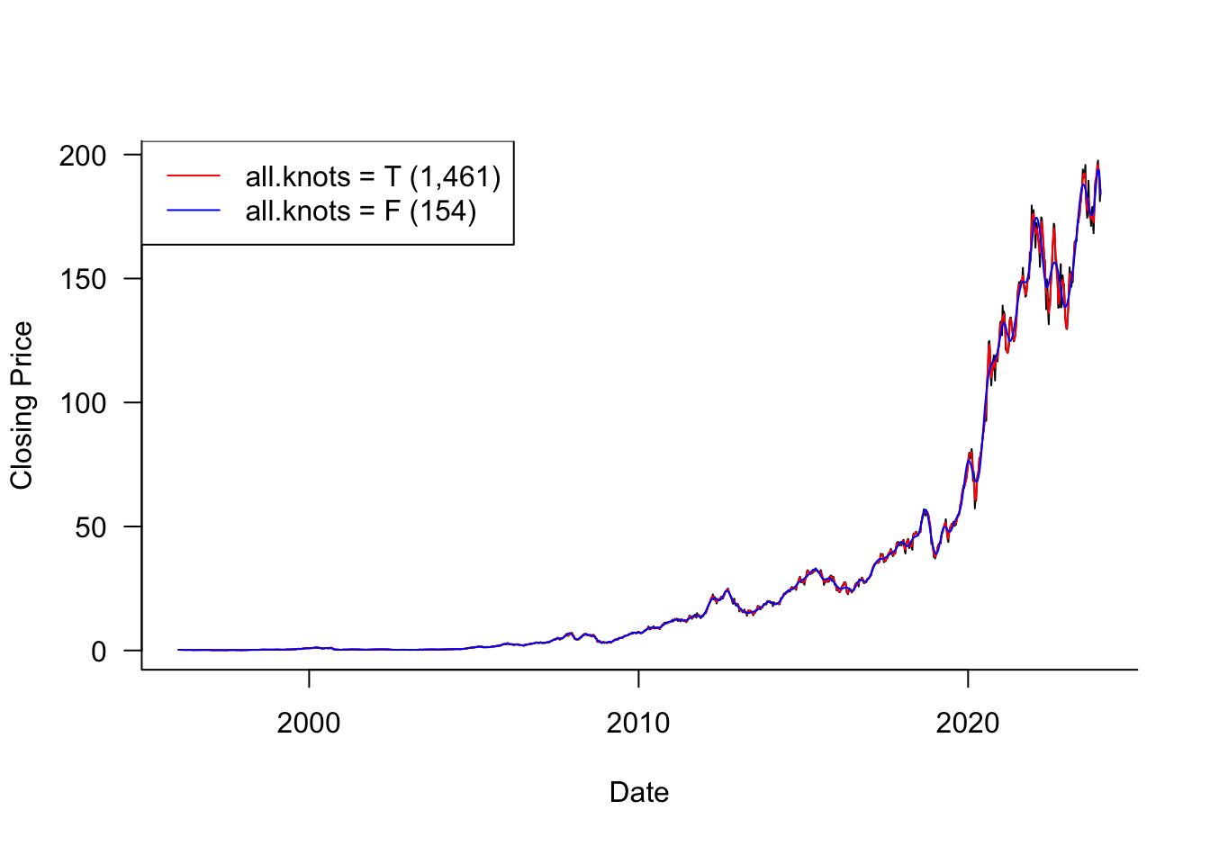
Figure 11.21 compares the fitted values for the smoothing splines. The smoothing spline from the second analysis does not capture the changes in share price in recent years but does a good job in the earlier years. The degree of smoothness in the weekly share prices changes over time which presents a challenge for any method that attempts to distill the degree of smoothness in a single parameter.
Several Python libraries provide smoothing functionality based on splines, for example pygam (LinearGam), sklearn (SplineTransformer), and scipy.interpolate (UnivariateSpline and make_smoothing_spline). The function that comes closest to the convenience of smooth.spline in R, which uses a penalized least squares approach and knot placements at all (or a large number) values of the input is make_smoothing_spline. The function performs generalized cross-validation to determine the optimal penalty parameter for the regularization term.
By not specifying the lam parameter of make_smoothing_spline, estimation of the penalty term by generalized cross-validation is invoked.
from scipy.interpolate import make_smoothing_spline

x = weekly['date']
y = weekly['Close']

spl = make_smoothing_spline(x,y)

plt.figure(figsize=(10, 6));
plt.plot(weekly['date'], weekly['Close'], color='black', linewidth=1.5);

plt.xlabel('Date');
plt.ylabel('Closing Price');

times = pd.date_range(x.min(), periods=1461, freq='1W')
plt.plot(times, spl(times), color='red', linewidth=0.5);

plt.grid(False);
plt.show();