18  Trees in Python

18.1 Packages

There are several libraries in Python for computing decision trees.

The scikit-learn library is the most widely used implementation for decision trees in Python. It provides comprehensive support for both classification and regression trees through the tree module. The main classes are DecisionTreeRegressor and DecisionTreeClassifier. These implementations follow the CART (Classification and Regression Trees) methodology of Breiman et al. (1984).

Some key features of scikit-learn’s tree implementations include: - Built-in support for cost-complexity pruning - Multiple criteria for measuring split quality (Gini impurity, entropy, MSE) - Handling of missing values through median imputation or custom strategies - Rich visualization options when combined with graphviz - Integration with the broader scikit-learn ecosystem for model selection and evaluation

The lightgbm and xgboost packages also implement decision trees as their base learners, though they are primarily used for gradient boosting rather than single trees. For this document, we’ll focus on scikit-learn as it provides the most straightforward implementation of CART-style trees.

18.2 Regression Trees

Basic Construction

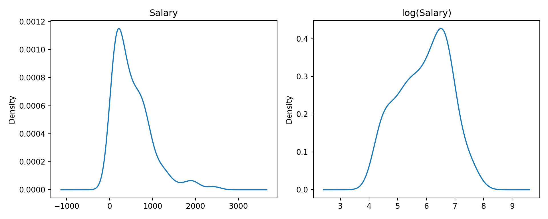
For this application we’ll use the Hitters data on performance and salaries of baseball players in the 1986/1987 seasons. Because the salaries are highly skewed, a log transformation is applied prior to constructing the tree (Figure 18.1).

import numpy as np
import pandas as pd
import matplotlib.pyplot as plt
import duckdb

con = duckdb.connect(database="ads.ddb", read_only=True)
hitters = con.sql("SELECT * FROM Hitters;").df().dropna()
con.close()

fig, (ax1, ax2) = plt.subplots(1, 2, figsize=(10, 4))
hitters['Salary'].plot.density(ax=ax1)
ax1.set_title('Salary')
np.log(hitters['Salary'].dropna()).plot.density(ax=ax2)
ax2.set_title('log(Salary)')
plt.tight_layout()
plt.show()
Figure 18.1: Salaries and log(Salaries) for the Hitters data.

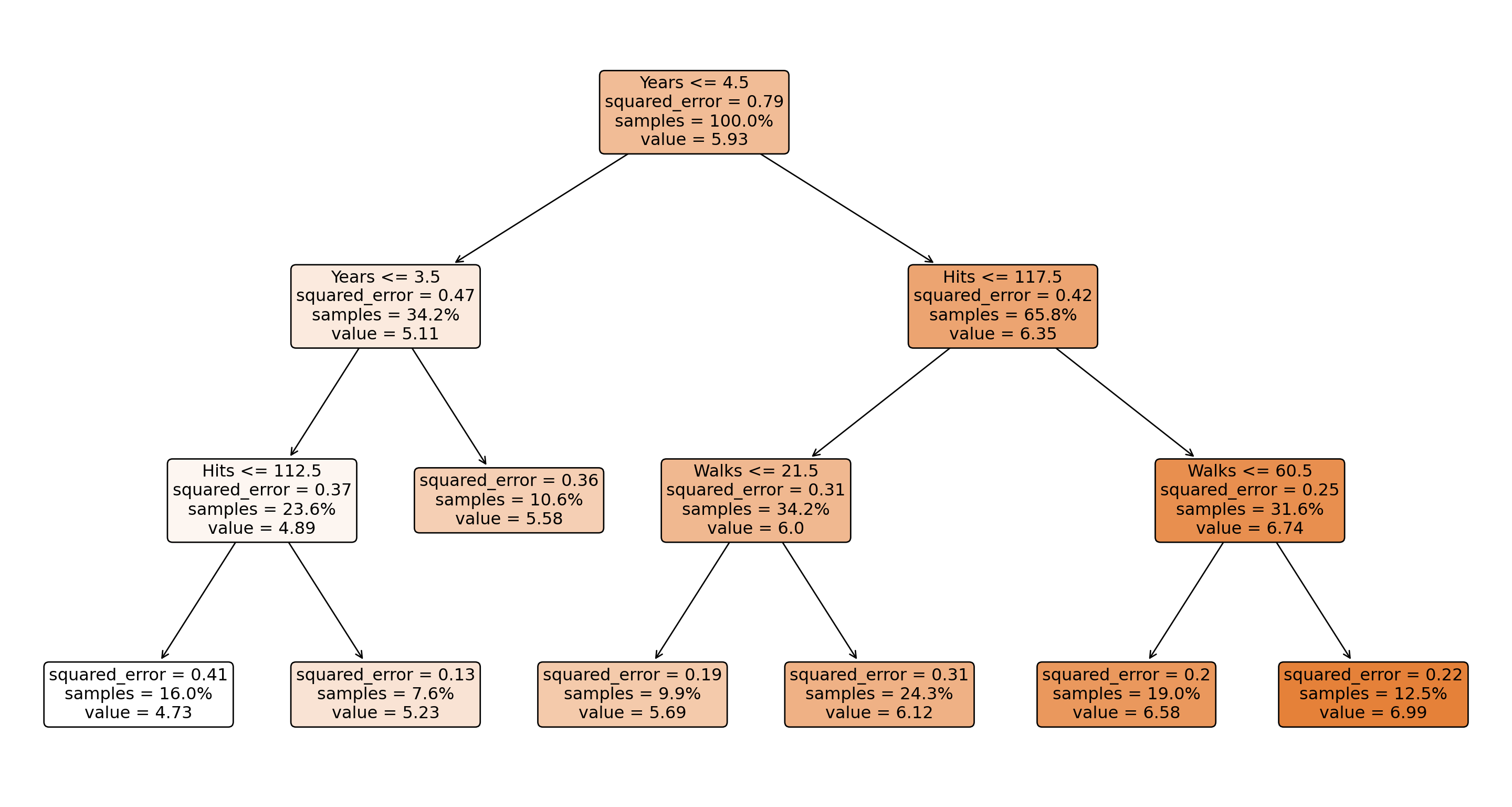
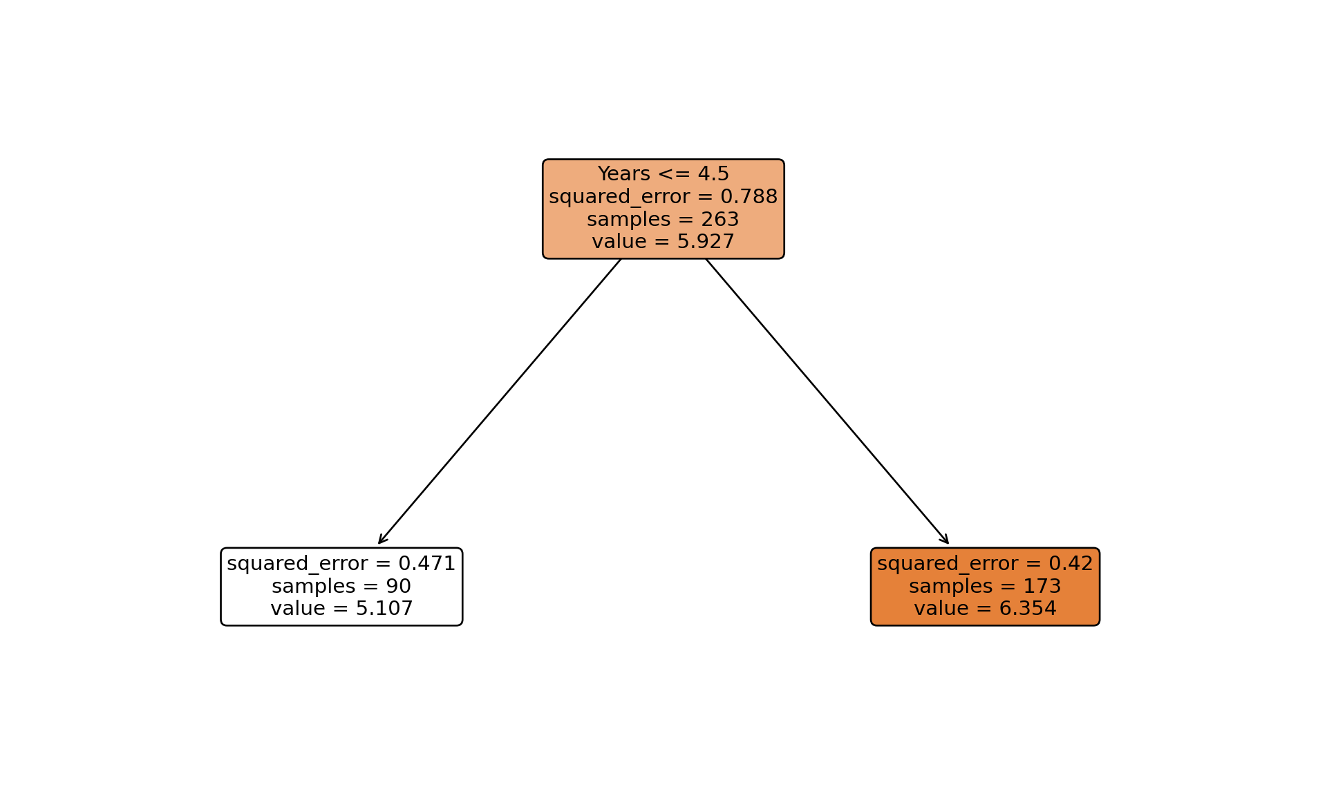
Now let’s fit a regression tree. We’ll use the same features as in the R example but with the scikit-learn implementation:

from sklearn.tree import DecisionTreeRegressor

features = [
    "Years",
    "Hits",
    "RBI",
    "Walks",
    "Runs",
    "HmRun",
    "PutOuts",
    "AtBat",
    "Errors",
]

X = hitters[features].fillna(0)
y = np.log(hitters["Salary"])

# Fit a simpler tree with controlled depth and minimum samples per leaf
t1 = DecisionTreeRegressor(
    max_depth=3,  # Limit tree depth to 3 levels
    min_samples_leaf=20,  # Require at least 20 samples per leaf
    random_state=87654,
)
t1.fit(X, y)
DecisionTreeRegressor(max_depth=3, min_samples_leaf=20, random_state=87654)
In a Jupyter environment, please rerun this cell to show the HTML representation or trust the notebook.
On GitHub, the HTML representation is unable to render, please try loading this page with nbviewer.org.
from sklearn.tree import plot_tree
plt.figure(figsize=(15, 8))
plot_tree(t1,
          feature_names=features,
          filled=True,
          rounded=True,
          fontsize=12,
          proportion=True,
          precision=2,
)
plt.tight_layout()
plt.show()
Figure 18.2: Simplified regression tree for log(salary) with controlled depth

Tree Summary

Unlike rpart in R, scikit-learn’s tree implementation doesn’t provide a built-in text summary. However, we can extract key information about the tree:

def print_tree_info(tree, feature_names):
    n_nodes = tree.tree_.node_count
    children_left = tree.tree_.children_left
    children_right = tree.tree_.children_right
    feature = tree.tree_.feature
    threshold = tree.tree_.threshold
    values = tree.tree_.value.squeeze()
    
    print(f"Total nodes: {n_nodes}")
    print(f"Number of leaves: {tree.get_n_leaves()}")
    print("\nFeature importance:")
    for name, imp in zip(feature_names, tree.feature_importances_):
        if imp > 0:  # Only show features that were used
            print(f"{name}: {imp:.3f}")
        
print_tree_info(t1, features)
Total nodes: 13
Number of leaves: 7

Feature importance:
Years: 0.749
Hits: 0.200
Walks: 0.051

Cross-validation and Pruning

Scikit-learn implements cost-complexity pruning through the ccp_alpha parameter. We can find the optimal alpha using cross-validation:

from sklearn.model_selection import cross_val_score

# Get alphas
path = t1.cost_complexity_pruning_path(X, y)
ccp_alphas = path.ccp_alphas

# Evaluate different alphas using cross-validation
mean_scores = []
std_scores = []

for ccp_alpha in ccp_alphas:
    tree = DecisionTreeRegressor(ccp_alpha=ccp_alpha, random_state=87654)
    scores = cross_val_score(tree, X, y, cv=10)
    mean_scores.append(scores.mean())
    std_scores.append(scores.std())

# Plot results
plt.figure(figsize=(10, 6))
plt.errorbar(ccp_alphas, mean_scores, yerr=std_scores, capsize=3)
plt.xlabel('ccp_alpha')
plt.ylabel('Mean cross-validation score')
plt.title('Cross-validation scores vs alpha')
plt.show()
Figure 18.3: Cross-validation scores vs complexity parameter alpha

We can then prune the tree using the optimal alpha value:

# Find optimal alpha (1-SE rule)
optimal_idx = np.argmax(mean_scores)
optimal_alpha = ccp_alphas[optimal_idx]

# Fit final tree
t_final = DecisionTreeRegressor(ccp_alpha=optimal_alpha, 
                               random_state=87654)
t_final.fit(X, y)
DecisionTreeRegressor(ccp_alpha=0.012516634191747047, random_state=87654)
In a Jupyter environment, please rerun this cell to show the HTML representation or trust the notebook.
On GitHub, the HTML representation is unable to render, please try loading this page with nbviewer.org.
Figure 18.4: Final pruned regression tree for Hitters data
# Visualize final tree
plt.figure(figsize=(15, 10))
plot_tree(t_final, 
          feature_names=features, 
          filled=True, 
          rounded=True, 
          fontsize=12)
plt.tight_layout()
plt.show()
Figure 18.5: Final pruned regression tree for Hitters data

Controlling the Tree

In scikit-learn, tree construction is controlled through parameters passed to the DecisionTreeRegressor constructor. Key parameters include:

  • min_samples_split: The minimum number of samples required to split a node (equivalent to minsplit in rpart)
  • min_samples_leaf: The minimum number of samples required in a leaf node (equivalent to minbucket in rpart)
  • max_depth: Maximum depth of the tree
  • ccp_alpha: Complexity parameter for pruning
  • criterion: The function to measure split quality (‘squared_error’, ‘friedman_mse’, ‘absolute_error’, ‘poisson’)

Fitting Stumps

To fit a stump (single-split tree), we simply set max_depth=1:

stump = DecisionTreeRegressor(max_depth=1, random_state=87654)
stump.fit(X, y)
DecisionTreeRegressor(max_depth=1, random_state=87654)
In a Jupyter environment, please rerun this cell to show the HTML representation or trust the notebook.
On GitHub, the HTML representation is unable to render, please try loading this page with nbviewer.org.
Figure 18.6: A stump fit to the Hitters data
plt.figure(figsize=(10, 6))
plot_tree(stump, 
          feature_names=features, 
          filled=True, 
          rounded=True, 
          fontsize=11)
plt.tight_layout()
plt.show()
Figure 18.7: A stump fit to the Hitters data

18.3 Classification Trees

Binary Classification

For binary classification, we’ll use the breast cancer data set from scikit-learn:

from sklearn.datasets import load_breast_cancer
from sklearn.tree import DecisionTreeClassifier

# Load data
cancer = load_breast_cancer()
X_cancer = pd.DataFrame(cancer.data, columns=cancer.feature_names)
y_cancer = pd.Series(cancer.target, name='malignant')

# Fit tree
clf = DecisionTreeClassifier(random_state=543, max_depth=3)  
clf.fit(X_cancer, y_cancer)
DecisionTreeClassifier(max_depth=3, random_state=543)
In a Jupyter environment, please rerun this cell to show the HTML representation or trust the notebook.
On GitHub, the HTML representation is unable to render, please try loading this page with nbviewer.org.
Figure 18.8: Classification tree for breast cancer data
# Visualize
plt.figure(figsize=(15, 10))
plot_tree(clf, 
          feature_names=list(cancer.feature_names), 
          class_names=['malignant', 'benign'],
          filled=True, 
          rounded=True, 
          fontsize=10)
plt.tight_layout()
plt.show()
Figure 18.9: Classification tree for breast cancer data
# Print accuracy
from sklearn.metrics import accuracy_score
print(f"Training accuracy: {accuracy_score(y_cancer, clf.predict(X_cancer)):.3f}")
Training accuracy: 0.979

Nominal Classification

For multi-class classification, we’ll use the iris data set:

from sklearn.datasets import load_iris

iris = load_iris()
X_iris = pd.DataFrame(iris.data, columns=iris.feature_names)
y_iris = pd.Series(iris.target, name='species')

multi_clf = DecisionTreeClassifier(random_state=543)
multi_clf.fit(X_iris, y_iris)
DecisionTreeClassifier(random_state=543)
In a Jupyter environment, please rerun this cell to show the HTML representation or trust the notebook.
On GitHub, the HTML representation is unable to render, please try loading this page with nbviewer.org.
Figure 18.10: Classification tree for iris data
plt.figure(figsize=(15, 10))
plot_tree(multi_clf, 
          feature_names=list(iris.feature_names),
          class_names=list(iris.target_names),
          filled=True, 
          rounded=True, 
          fontsize=11)
plt.tight_layout()
plt.show()
Figure 18.11: Classification tree for iris data
# Print accuracy
print(f"Training accuracy: {accuracy_score(y_iris, multi_clf.predict(X_iris)):.3f}")
Training accuracy: 1.000
Note

All tree visualizations in this document use plt.tight_layout() to prevent node overlap, and the figures are sized appropriately to ensure readability. The fontsize parameter in plot_tree is adjusted based on the complexity of the tree.