4  Parameter Estimation

4.1 Introduction

Statistical models contain two types of unknown quantities, parameters and hyperparameters. Parameters describe the distributional properties of the data; they are part of the mean function or the variance-covariance structure of the model. They are estimated from the data.

This chapter is not concerned with tuning hyperparameters but with the principles we use to estimate parameters of a model’s mean function from data—that is, estimating the internal parameters of the model.

Finding parameter estimates can be expressed as a numerical problem: find the values that minimize some metric of discrepancy between data and the model. The discrepancy can be some measure of loss such as squared error between observed and predicted target values \[\left( y_i - \widehat{f}_i(\textbf{x};\boldsymbol{\theta}) \right)^2\] or the misclassification error \[ I(y_i \ne \widehat{f}_i(\textbf{x};\boldsymbol{\theta})) \] and the loss for the entire data set is summed over all observations, for example \[ \ell(\textbf{y};\boldsymbol{\theta}) = \sum_{i=1}^n \left( y_i - \widehat{y}_i \right)^2 \]

The solution to the minimization problem \[ \mathop{\mathrm{arg\,min}}_\boldsymbol{\theta}\, \ell(\textbf{y};\boldsymbol{\theta}) \] is the estimator \(\widehat{\boldsymbol{\theta}}\) of the parameters \(\boldsymbol{\theta}\).

In some situations, this minimization problem has a closed-form solution that can be computed directly. In other cases we have to rely on numerical procedures to find a solution iteratively or approximations to simplify a complex or intractable problem. The solution \(\widehat{\boldsymbol{\theta}}\) is unique for some problems and might be one of many solutions, not all equally good.

Expressing parameter estimation as a general minimization problem does not reveal the foundations of important principles in parameter estimation, in particular, least squares and maximum likelihood estimation. We introduce these principles based on geometric and probabilistic considerations, the relationship to function minimization will be obvious.

Note

All optimization tasks will be presented as minimization problem. Finding the maximum of a function can be turned into a minimization of its negative value.

4.2 Least Squares Estimation

Least squares estimation is arguably one of the most important estimation principles and rests on a geometric concept. Suppose we have a model with additive errors, \(\textbf{Y}= \mathbf{f}(\textbf{x}; \boldsymbol{\theta}) + \boldsymbol{\epsilon}\). The function \(\mathbf{f}()\) is an \((n \times 1)\) vector of the mean function evaluations, the \(i\)th value is \(f(\textbf{x}_i;\boldsymbol{\theta})\). The least squares estimate \(\widehat{\boldsymbol{\theta}}\) of \(\boldsymbol{\theta}\) is the value that is closest to \(\textbf{Y}\) among all possible values \(\tilde{\boldsymbol{\theta}}\).

Ordinary Least Squares (OLS)

Consider the identity

\[ \textbf{Y}= \textbf{f}(\textbf{x};\tilde{\boldsymbol{\theta}}) + \left(\textbf{Y}- \textbf{f}(\textbf{x};\tilde{\boldsymbol{\theta}}) \right) \]

that expresses the observed data \(\textbf{Y}\) as the sum of fitted values and residuals.

By the Pythagorean theorem, the solution \(\widehat{\boldsymbol{\theta}}\) with the smallest vector of residuals is the orthogonal projection of \(\textbf{Y}\) onto \(\textbf{f}\), which implies that \[ \left(\textbf{Y}- \textbf{f}(\textbf{x};\widehat{\boldsymbol{\theta}}) \right)^\prime \textbf{f}(\textbf{x};\widehat{\boldsymbol{\theta}}) = \textbf{0} \] When \(\textbf{f}(\textbf{x};\boldsymbol{\theta})\) is linear in the parameters, it is common to denote the coefficients (parameters) as \(\boldsymbol{\beta}\) instead of the more generic \(\boldsymbol{\theta}\). We thus write the standard linear (regression) as \[ \textbf{Y}= \textbf{X}\boldsymbol{\beta}+ \boldsymbol{\epsilon} \] and the orthogonality criterion becomes \[ \left(\textbf{Y}- \textbf{X}\widehat{\boldsymbol{\beta}}\right)^\prime \textbf{X}\widehat{\boldsymbol{\beta}} = \textbf{0} \] It is easy to show that this implies \[ \textbf{X}^\prime\textbf{X}\widehat{\boldsymbol{\beta}} = \textbf{X}^\prime\textbf{Y} \] and if the cross-product matrix \(\textbf{X}^\prime\textbf{X}\) is of full rank, the (ordinary) least squares estimator is \[ \widehat{\boldsymbol{\beta}} = (\textbf{X}^\prime\textbf{X})^{-1}\textbf{X}^\prime\textbf{Y} \] Expressed as the problem of minimizing a loss function, ordinary least squares (OLS) is approached as follows. Suppose that we measure loss as squared-error loss \((y_i - \widehat{y}_i)^2\). In the linear model where \(\widehat{y}_i = \textbf{x}_i^\prime \widehat{\boldsymbol{\beta}}\), the loss function is the residual (error) sum of squares \[ \text{SSE}(\boldsymbol{\beta}) = \boldsymbol{\epsilon}^\prime\boldsymbol{\epsilon}= \left( \textbf{Y}-\textbf{X}^\prime\boldsymbol{\beta}\right)^\prime \left(\textbf{Y}-\textbf{X}^\prime\boldsymbol{\beta}\right) \] and the minimization problem is \[ \mathop{\mathrm{arg\,min}}_\boldsymbol{\beta}\, \text{SSE}(\boldsymbol{\beta}) \]

To find the minimum we set to zero the derivative of \(\text{SSE}(\boldsymbol{\beta})\) with respect to \(\boldsymbol{\beta}\). Expanding the residual sum of squares yields \[ SSE(\boldsymbol{\beta}) = \textbf{Y}^\prime\textbf{Y}- 2\boldsymbol{\beta}^\prime\textbf{X}^\prime\textbf{Y}+ \boldsymbol{\beta}^\prime\textbf{X}^\prime\textbf{X}\boldsymbol{\beta} \]

The derivative (Section 3.5) with respect to \(\boldsymbol{\beta}\) is \[ \frac{\partial\,\text{SSE}(\boldsymbol{\beta})}{\partial\boldsymbol{\beta}} = -2\textbf{X}^\prime\textbf{Y}+ 2\textbf{X}^\prime\textbf{X}\boldsymbol{\beta} \]

Setting the derivative to zero and solving yields the normal equations as above: \[ \textbf{X}^\prime\textbf{X}\widehat{\boldsymbol{\beta}} = \textbf{X}^\prime\textbf{Y} \] and the OLS estimator \[ \widehat{\boldsymbol{\beta}} = (\textbf{X}^\prime\textbf{X})^{-1}\textbf{X}^\prime\textbf{Y} \] The vector of fitted values, \(\widehat{\textbf{y}}\) is obtained by pre-multiplying with the data matrix

\[\begin{align*} \widehat{\textbf{Y}} &= \textbf{X}^\prime\widehat{\boldsymbol{\beta}} = (\textbf{X}^\prime\textbf{X})^{-1}\textbf{X}^\prime\textbf{Y}\\ &= \textbf{H}\textbf{Y} \end{align*}\]

The matrix \(\textbf{H}\) is called the “Hat” matrix, because pre-multiplying \(\textbf{Y}\) with \(\textbf{H}\) “puts hats on the \(y\)s” (Section 3.6.2). The last equation shows that the OLS estimator is a linear estimator, \(\widehat{y}_i\) is a linear combination of all \(y_i\), the weights of the linear combination are given by the entries of the hat matrix.

The statistical properties of the OLS estimator depend on the nature of the random error process. The most common assumption is that the \(\epsilon_i\) have zero mean and are iid, independently and identically distributed, formally, \(\boldsymbol{\epsilon}\sim (\textbf{0},\sigma^2\textbf{I})\).

Note

The statement \(\boldsymbol{\epsilon}\sim (\textbf{0},\sigma^2\textbf{I})\) is technically weaker than stating independence, it implies zero correlations among the observations. Independent random variables are uncorrelated, but the reverse is not necessarily true. You can conclude independence from lack of correlations for Gaussian (normal) random variables, but not generally.

In the iid case, the OLS estimator is unbiased, \(\text{E}[\widehat{\boldsymbol{\beta}}] = \boldsymbol{\beta}\) and has variance \(\text{Var}[\widehat{\boldsymbol{\beta}}] = \sigma^2(\textbf{X}^\prime\textbf{X})^{-1}\). In fact, it is a BLUE (best linear unbiased estimator) in this situation. No other unbiased estimator has smaller variance than the OLS estimator. However, it is possible that other estimators have smaller mean squared error than the OLS estimator, if the introduction of bias is more than offset by a reduction of the variance of the estimator. This is important in high-dimensional problems where the number of predictors (\(p\)) is large. As \(p\) increases, the OLS estimator becomes more unstable, especially if the predictors are highly related to each other (a condition known as multi-collinearity). The values of \(\widehat{\boldsymbol{\beta}}\) then have a tendency to vary widely. Estimators that limit the variability of the model coefficients through regularization techniques, such as Ridge or Lasso regression, can have considerably lower variance at the expense of some bias, leading to better mean squared error.

Note

A Gaussian distribution (normality) assumption is not a requirement of the linear model or of least squares estimation. The OLS estimator has desirable properties even if the errors are not normally distributed. However, making statements about the significance of the \(\beta_j\) requires additional assumptions such as \(\boldsymbol{\epsilon}\sim G(\textbf{0},\sigma^2\textbf{I})\).

When \(\boldsymbol{\epsilon}\sim G(\textbf{0},\sigma^2\textbf{I})\), the OLS estimator is not only BLUE but a minimum variance unbiased estimator (MVUE), best among all unbiased estimators, not only those estimators linear in \(\textbf{Y}\).

Least squares from scratch

To understand statistical computing, it is a good idea to implement some algorithms from scratch. That also helps to identify the numbers reported by statistical software. Here we implement the OLS estimator from scratch in R using the fitness data set. The data comprise measurements of aerobic capacity and other attributes on 31 men involved in a physical fitness course at N.C. State University.

Aerobic capacity is the ability of the heart and lungs to provide the body with oxygen. It is a measure of fitness and expressed as the oxygen intake in ml per kg body weight per minute. Measuring aerobic capacity is expensive and time consuming compared to attributes such as age, weight, and pulse. The question is whether aerobic capacity can be predicted from the easily measurable attributes. If so, a predictive equation can reduce time and effort to assess aerobic capacity.

The variables are

  • Age: age in years
  • Weight: weight in kg
  • Oxygen: oxygen intake rate (ml per kg body weight per minute)
  • RunTime: time to run 1.5 miles (minutes)
  • RestPulse: heart rate while resting
  • RunPulse: heart rate while running (same time Oxygen rate measured)
  • MaxPulse: maximum heart rate recorded while running

The linear model we have in mind is \[ \text{Oxygen}_i = \beta_0 + \beta_1\text{Age}_i + \beta_2\text{Weight}_i + \beta_3\text{RunTime}_i + \beta_4\text{RestPulse}_i + \beta_5\text{RunPulse}_i + \beta_6\text{MaxPulse}_i + \epsilon_i \] and the \(\epsilon_i\) are assumed zero-mean random variables with common variance \(\sigma^2\).

The following code loads the data from the ads DuckDB database.

library("duckdb")

con <- dbConnect(duckdb(),dbdir = "ads.ddb",read_only=TRUE)
fit <- dbGetQuery(con, "SELECT * FROM fitness")
dbDisconnect(con)

head(fit)
  Age Weight Oxygen RunTime RestPulse RunPulse MaxPulse
1  44  89.47 44.609   11.37        62      178      182
2  40  75.07 45.313   10.07        62      185      185
3  44  85.84 54.297    8.65        45      156      168
4  42  68.15 59.571    8.17        40      166      172
5  38  89.02 49.874    9.22        55      178      180
6  47  77.45 44.811   11.63        58      176      176
import duckdb

con = duckdb.connect(database="ads.ddb", read_only=True)
fit = con.sql("SELECT * FROM fitness").df()
con.close()

fit.head()
   Age  Weight  Oxygen  RunTime  RestPulse  RunPulse  MaxPulse
0   44   89.47  44.609    11.37         62       178       182
1   40   75.07  45.313    10.07         62       185       185
2   44   85.84  54.297     8.65         45       156       168
3   42   68.15  59.571     8.17         40       166       172
4   38   89.02  49.874     9.22         55       178       180

The target variable for the linear model is Oxygen, the remaining variables are inputs to the regression. The next statements create the \(\textbf{y}\) vector and the \(\textbf{X}\) matrix for the model. Note that the first column of \(\textbf{X}\) is a vector of ones, representing the “input” for the intercept \(\beta_0\).

y <- as.matrix(fit[,which(names(fit)=="Oxygen")])
X <- as.matrix(cbind(Intcpt=rep(1,nrow(fit)), 
                     fit[,which(names(fit)!="Oxygen")]))
head(X)
     Intcpt Age Weight RunTime RestPulse RunPulse MaxPulse
[1,]      1  44  89.47   11.37        62      178      182
[2,]      1  40  75.07   10.07        62      185      185
[3,]      1  44  85.84    8.65        45      156      168
[4,]      1  42  68.15    8.17        40      166      172
[5,]      1  38  89.02    9.22        55      178      180
[6,]      1  47  77.45   11.63        58      176      176
import pandas as pd
import numpy as np

y = fit[['Oxygen']].values

# First create a column of 1s for the intercept
intercept = np.ones((len(fit), 1))

# Get all columns except Oxygen
X_without_intercept = fit.drop('Oxygen', axis=1).values

# Combine intercept and other columns and add column names
X = np.hstack((intercept, X_without_intercept))
X_column_names = ['Intcpt'] + list(fit.drop('Oxygen', axis=1).columns)

print("First few rows of X:")
First few rows of X:
print(X[:5, :])  
[[  1.    44.    89.47  11.37  62.   178.   182.  ]
 [  1.    40.    75.07  10.07  62.   185.   185.  ]
 [  1.    44.    85.84   8.65  45.   156.   168.  ]
 [  1.    42.    68.15   8.17  40.   166.   172.  ]
 [  1.    38.    89.02   9.22  55.   178.   180.  ]]
print("Column names:", X_column_names)
Column names: ['Intcpt', 'Age', 'Weight', 'RunTime', 'RestPulse', 'RunPulse', 'MaxPulse']

Next we are building the \(\textbf{X}^\prime\textbf{X}\) matrix and compute its inverse, \((\textbf{X}^\prime\textbf{X})^{-1}\), with the solve() function. t() transposes a matrix and %*% indicates that we are performing matrix multiplication rather than elementwise multiplication.

XpX <- t(X) %*% X
XpXInv <- solve(XpX)

Next we are building the \(\textbf{X}^\prime\textbf{X}\) matrix and compute its inverse, \((\textbf{X}^\prime\textbf{X})^{-1}\), with the np.linalg.inv() function. .T transposes a matrix and @ indicates that we are performing matrix multiplication rather than elementwise multiplication.

XpX = X.T @ X
# Alternative: XpX = np.matmul(X.T, X)

XpXInv = np.linalg.inv(XpX)

We can verify that XpxInv is indeed the inverse of XpX by multiplying the two. This should yield the identity matrix

round(XpX %*% XpXInv,3)
          Intcpt Age Weight RunTime RestPulse RunPulse MaxPulse
Intcpt         1   0      0       0         0        0        0
Age            0   1      0       0         0        0        0
Weight         0   0      1       0         0        0        0
RunTime        0   0      0       1         0        0        0
RestPulse      0   0      0       0         1        0        0
RunPulse       0   0      0       0         0        1        0
MaxPulse       0   0      0       0         0        0        1
np.round(XpX @ XpXInv,3)
array([[ 1.,  0., -0.,  0.,  0., -0.,  0.],
       [-0.,  1.,  0.,  0.,  0.,  0., -0.],
       [ 0.,  0.,  1.,  0.,  0., -0.,  0.],
       [-0.,  0., -0.,  1.,  0., -0.,  0.],
       [-0.,  0., -0.,  0.,  1., -0.,  0.],
       [-0.,  0., -0.,  0.,  0.,  1.,  0.],
       [-0., -0., -0.,  0.,  0., -0.,  1.]])

Next we compute the OLS estimate of \(\boldsymbol{\beta}\) and the predicted values \(\widehat{\textbf{y}} = \textbf{X}\widehat{\boldsymbol{\beta}}\).

beta_hat <- XpXInv %*% t(X) %*% y
beta_hat
                  [,1]
Intcpt    102.93447948
Age        -0.22697380
Weight     -0.07417741
RunTime    -2.62865282
RestPulse  -0.02153364
RunPulse   -0.36962776
MaxPulse    0.30321713
y_hat <- X %*% beta_hat
beta_hat = XpXInv @ X.T @ y
print(beta_hat)
[[ 1.02934479e+02]
 [-2.26973796e-01]
 [-7.41774137e-02]
 [-2.62865282e+00]
 [-2.15336398e-02]
 [-3.69627758e-01]
 [ 3.03217129e-01]]

y_hat = X @ beta_hat

The estimate of the intercept is \(\widehat{\beta}_0\) = 102.9344795, the estimate of the coefficient for Age is \(\widehat{\beta}_1\) = -0.2269738 and so on.

The residuals \(\widehat{\boldsymbol{\epsilon}} = \textbf{y}- \widehat{\textbf{y}}\), the error sum of squares

\[ \text{SSE} = (\textbf{y}- \widehat{\textbf{y}} )^\prime (\textbf{y}- \widehat{\textbf{y}}) = \sum_{i=1}^n \left(y_i - \widehat{y}_i\right)^2 \] and the estimate of the residual variance \[ \widehat{\sigma}^2 = \frac{1}{n-r(\textbf{X})} \, \text{SSE} \]

are computed as

library("Matrix")

residuals <- y - y_hat
SSE <- sum(residuals^2)
n <- nrow(fit)
rankX <- rankMatrix(XpX)[1]
sigma2_hat <- SSE/(n - rankX)

SSE
[1] 128.8379
sigma2_hat
[1] 5.368247

We used the rankMatrix function in the Matrix package to compute the rank of \(\textbf{X}\), which is identical to the rank of \(\textbf{X}^\prime\textbf{X}\).

residuals = y - y_hat

SSE = np.sum(residuals**2)
n = len(fit)
rankX = np.linalg.matrix_rank(XpX)
sigma2_hat = SSE / (n - rankX)

print(f"SSE: {SSE:.4f}")
SSE: 128.8379
print(f"sigma2_hat: {sigma2_hat:.4f}")
sigma2_hat: 5.3682

With these quantities available, the variance-covariance matrix of \(\widehat{\boldsymbol{\beta}}\), \[ \text{Var}[\widehat{\boldsymbol{\beta}}] = \sigma^2 (\textbf{X}^\prime\textbf{X})^{-1} \] can be estimated by substituting \(\widehat{\sigma}^2\). The standard errors of the regression coefficient estimates are the square roots of the diagonal values of this matrix.

Var_beta_hat <- sigma2_hat * XpXInv
se_beta_hat <- sqrt(diag(Var_beta_hat))
se_beta_hat
     Intcpt         Age      Weight     RunTime   RestPulse    RunPulse 
12.40325810  0.09983747  0.05459316  0.38456220  0.06605428  0.11985294 
   MaxPulse 
 0.13649519 
Var_beta_hat = sigma2_hat * XpXInv
se_beta_hat = np.sqrt(np.diag(Var_beta_hat))
print(se_beta_hat)
[12.4032581   0.09983747  0.05459316  0.3845622   0.06605428  0.11985294
  0.13649519]

Now let’s compare our results to the output from the lm() function.

linmod <- lm(Oxygen ~ ., data=fit)
summary(linmod)

Call:
lm(formula = Oxygen ~ ., data = fit)

Residuals:
    Min      1Q  Median      3Q     Max 
-5.4026 -0.8991  0.0706  1.0496  5.3847 

Coefficients:
             Estimate Std. Error t value Pr(>|t|)    
(Intercept) 102.93448   12.40326   8.299 1.64e-08 ***
Age          -0.22697    0.09984  -2.273  0.03224 *  
Weight       -0.07418    0.05459  -1.359  0.18687    
RunTime      -2.62865    0.38456  -6.835 4.54e-07 ***
RestPulse    -0.02153    0.06605  -0.326  0.74725    
RunPulse     -0.36963    0.11985  -3.084  0.00508 ** 
MaxPulse      0.30322    0.13650   2.221  0.03601 *  
---
Signif. codes:  0 '***' 0.001 '**' 0.01 '*' 0.05 '.' 0.1 ' ' 1

Residual standard error: 2.317 on 24 degrees of freedom
Multiple R-squared:  0.8487,    Adjusted R-squared:  0.8108 
F-statistic: 22.43 on 6 and 24 DF,  p-value: 9.715e-09

Based on the quantities calculated earlier, the following code reproduces the lm summary in R.

tvals <- beta_hat/se_beta_hat
pvals <- 2*(1-pt(abs(tvals),n-rankX))
result <- cbind(beta_hat, se_beta_hat, tvals, pvals)
colnames(result) <- c("Estimate", "Std. Error", "t value", "Pr(>|t|)")
round(result,5)
           Estimate Std. Error  t value Pr(>|t|)
Intcpt    102.93448   12.40326  8.29899  0.00000
Age        -0.22697    0.09984 -2.27343  0.03224
Weight     -0.07418    0.05459 -1.35873  0.18687
RunTime    -2.62865    0.38456 -6.83544  0.00000
RestPulse  -0.02153    0.06605 -0.32600  0.74725
RunPulse   -0.36963    0.11985 -3.08401  0.00508
MaxPulse    0.30322    0.13650  2.22145  0.03601
cat("\nResidual standard error: ", sqrt(sigma2_hat)," on ", n-rankX, "degrees of freedom\n")

Residual standard error:  2.316948  on  24 degrees of freedom
SST <- sum( (y -mean(y))^2 )
cat("Multiple R-squared: ", 1-SSE/SST, 
    "Adjusted R-squared: ", 1 - (SSE/SST)*(n-1)/(n-rankX), "\n")
Multiple R-squared:  0.8486719 Adjusted R-squared:  0.8108399 
Fstat <- ((SST-SSE)/(rankX-1)) / (SSE/(n-rankX))
cat("F-statistic: ", Fstat, "on ", 
    rankX-1, "and", n-rankX, "DF, p-value:", 1-pf(Fstat,rankX-1,n-rankX))
F-statistic:  22.43263 on  6 and 24 DF, p-value: 9.715305e-09

Now let’s compare our results to the output to the ordinary least squares fit in statsmodels.

import statsmodels.api as sm

X = sm.add_constant(fit.drop('Oxygen', axis=1))
y = fit['Oxygen']

# Fit the model
linmod = sm.OLS(y, X).fit()

print(linmod.summary())
                            OLS Regression Results                            
==============================================================================
Dep. Variable:                 Oxygen   R-squared:                       0.849
Model:                            OLS   Adj. R-squared:                  0.811
Method:                 Least Squares   F-statistic:                     22.43
Date:                Wed, 30 Apr 2025   Prob (F-statistic):           9.72e-09
Time:                        17:23:10   Log-Likelihood:                -66.068
No. Observations:                  31   AIC:                             146.1
Df Residuals:                      24   BIC:                             156.2
Df Model:                           6                                         
Covariance Type:            nonrobust                                         
==============================================================================
                 coef    std err          t      P>|t|      [0.025      0.975]
------------------------------------------------------------------------------
const        102.9345     12.403      8.299      0.000      77.335     128.534
Age           -0.2270      0.100     -2.273      0.032      -0.433      -0.021
Weight        -0.0742      0.055     -1.359      0.187      -0.187       0.038
RunTime       -2.6287      0.385     -6.835      0.000      -3.422      -1.835
RestPulse     -0.0215      0.066     -0.326      0.747      -0.158       0.115
RunPulse      -0.3696      0.120     -3.084      0.005      -0.617      -0.122
MaxPulse       0.3032      0.136      2.221      0.036       0.022       0.585
==============================================================================
Omnibus:                        2.609   Durbin-Watson:                   1.711
Prob(Omnibus):                  0.271   Jarque-Bera (JB):                1.465
Skew:                          -0.069   Prob(JB):                        0.481
Kurtosis:                       4.056   Cond. No.                     7.91e+03
==============================================================================

Notes:
[1] Standard Errors assume that the covariance matrix of the errors is correctly specified.
[2] The condition number is large, 7.91e+03. This might indicate that there are
strong multicollinearity or other numerical problems.

# If you want to access specific components:
# print("Coefficients:", linmod.params)
# print("Standard errors:", linmod.bse)
# print("R-squared:", linmod.rsquared)

Weighted and Generalized Least Squares

Another interesting feature of the OLS estimator is that it does not depend on the variability of the model errors. Whether \(\sigma^2\) is large or small, the OLS estimator is only a function of \(\textbf{Y}\) and \(\textbf{X}\). However, the error variance affects the variability of \(\widehat{\boldsymbol{\beta}}\).

When the error distribution is more complex than the iid case, the variance and covariances of the errors must be taken into account for least squares estimators to retain their optimality. The first case is that of uncorrelated errors that have unequal variances, a situation known as heteroscedasticity. The variance-covariance matrix of the \(\boldsymbol{\epsilon}\) is then a diagonal matrix. Let’s call the inverse of the variance-covariance matrix \(\textbf{W}\). \(\textbf{W}\) is a \((n \times n)\) d iagonal matrix with \(1/\sigma^2_i\), the inverse of the variance of the \(i\)th observation, in the \(i\)th diagonal cell. The weighted least squares estimator \[ \widehat{\boldsymbol{\beta}}_{WLS} = (\textbf{X}^\prime\textbf{W}\textbf{X})^{-1}\textbf{X}^\prime\textbf{W}\textbf{Y} \] is the optimal estimator in this situation.

Tip

A weighted analysis is the correct approach when the weights are inversely proportional to the variance of the observations. This makes sense if we think of the weights as expressing how strongly the analysis should depend on a particular observation. A larger variance means that we are less certain about the observed value and thus should give the observation less weight.

In the weighted model the variance-covariance matrix of the errors are diagonal, the observations have unequal variances but are uncorrelated. If the errors are correlated, the variance-covariance matrix is not diagonal. Suppose that \(\boldsymbol{\epsilon}\sim (\textbf{0}, \textbf{V})\), the optimal least squares estimator is the generalized least squares estimator \[ \widehat{\boldsymbol{\beta}}_{GLS} = (\textbf{X}^\prime\textbf{V}^{-1}\textbf{X})^{-1}\textbf{X}^\prime\textbf{V}^{-1}\textbf{Y} \]

This seems like a small change from the weighted case, replacing \(\textbf{W}\) with \(\textbf{V}\). So what is the big deal? In weighted analyses the weights are often known, at least up to a multiple. For example, when the variability of the target variable increases proportionally with one of the inputs, \(x_2\) say, then \(\textbf{W}\) is essentially known. In situations where we apply GLS estimation, \(\textbf{V}\) is often not known and depends itself on parameters. The overall model then composes a model for the mean function that depends on \(\boldsymbol{\beta}\) and a model for the error structure that depends on \(\boldsymbol{\theta}\):

\[\begin{align*} \textbf{Y}&= \textbf{X}\boldsymbol{\beta}+ \boldsymbol{\epsilon}\\ \boldsymbol{\epsilon}& \sim (\textbf{0}, \textbf{V}(\boldsymbol{\theta})) \end{align*}\]

and both sets of parameters must be derived from the data. This is somewhat of a cat-and-mouse game. You need to know \(\boldsymbol{\beta}\) to estimate \(\boldsymbol{\theta}\) and the estimates of \(\boldsymbol{\theta}\) depend on \(\boldsymbol{\beta}\). This tension is resolved by the estimated generalized least squares principle. Given an estimate of \(\boldsymbol{\theta}\), you compute the estimated GLS estimator \[ \widehat{\boldsymbol{\beta}}_{EGLS} = (\textbf{X}^\prime\textbf{V}(\widehat{\boldsymbol{\theta}})^{-1}\textbf{X})^{-1}\textbf{X}^\prime\textbf{V}(\widehat{\boldsymbol{\theta}})^{-1}\textbf{Y} \]

With an updated estimate of \(\boldsymbol{\beta}\) you use a different estimation principle to compute an updated estimate of \(\boldsymbol{\theta}\). This is the principle behind restricted maximum likelihood, a likelihood-based estimation principle important for mixed models.

Nonlinear Least Squares

The linear structure of the model \(\textbf{Y}= \textbf{X}\boldsymbol{\beta}+ \boldsymbol{\epsilon}\) leads to a closed form solution of the least squares problem \[ \widehat{\boldsymbol{\beta}} = (\textbf{X}^\prime\textbf{X})^{-1}\textbf{X}^\prime\textbf{Y} \]

When the model is nonlinear in the parameters, \(\textbf{Y}= \textbf{f}(\textbf{x};\boldsymbol{\theta}) + \boldsymbol{\epsilon}\), finding the solution that minimizes

\[ \text{SSE} = \left(\textbf{Y}- \textbf{f}(\textbf{x};\boldsymbol{\theta})\right)^\prime \left(\textbf{Y}- \textbf{f}(\textbf{x};\boldsymbol{\theta})\right) \tag{4.1}\]

is not so straightforward, it requires an iterative approach. Starting from some initial guess for \(\boldsymbol{\theta}\), call it \(\widehat{\boldsymbol{\theta}}^{(0)}\), we iteratively update the guess until we have arrived at step \(t\) at \(\widehat{\boldsymbol{\theta}}^{(t)}\) such that \[ \frac{\partial \,\text{SSE}}{\partial\boldsymbol{\theta}} \lvert_{\widehat{\boldsymbol{\theta}}^{(t)}} = \textbf{0} \] The left hand side of the previous expression is read as the derivative of SSE with respect to \(\boldsymbol{\theta}\), evaluated at \(\widehat{\boldsymbol{\theta}}^{t}\).

Common iterative approaches to solve this optimization problem involve the Gauss-Newton and Newton-Raphson algorithms. We introduce the Gauss-Newton method here. The basic idea is that we can approximate the nonlinear mean function with a linear version that depends on some current values for \(\boldsymbol{\theta}\). Linear least squares can be applied to the linearized form to compute an update of the estimate for \(\boldsymbol{\theta}\). With the updated estimate the approximation can be refined and another least squares step is performed. This sequence is repeated until some convergence criterion is met.

We start by approximating \(\textbf{f}(\textbf{x};\boldsymbol{\theta})\) with a first-order Taylor series about \(\boldsymbol{\theta}^{(0)}\) \[ \textbf{f}(\textbf{x}; \boldsymbol{\theta}) \approx \textbf{f}(\textbf{x};\boldsymbol{\theta}^{(0)}) + \textbf{F}^{(0)}(\boldsymbol{\theta}-\boldsymbol{\theta}^{(0)}) \] where \(\textbf{F}^{(0)}\) is a matrix of derivatives of \(\textbf{f}(\textbf{x};\boldsymbol{\theta})\) evaluated at the value \(\boldsymbol{\theta}^{(0)}\). The residual \(\textbf{y}- \textbf{f}(\textbf{x};\boldsymbol{\theta})\) can now be approximated as \(\textbf{r}(\boldsymbol{\theta}^{(0)}) = \textbf{y}- \textbf{f}(\textbf{x};\boldsymbol{\theta}^{(0)}) - \textbf{F}^{(0)}(\boldsymbol{\theta}- \boldsymbol{\theta}^{(0)})\). Substitute this expression into Equation 4.1 we get an approximate error sums of squares

\[ \text{SSE} \approx \textbf{r}(\boldsymbol{\theta}^{(0)})^\prime \textbf{r}(\boldsymbol{\theta}^{(0)}) - 2 \textbf{r}(\boldsymbol{\theta}^{(0)})\textbf{F}^{(0)}(\boldsymbol{\theta}- \boldsymbol{\theta}^{(0)}) + (\boldsymbol{\theta}- \boldsymbol{\theta}^{(0)})^\prime \textbf{F}^{(0)\prime}\textbf{F}^{(0)} (\boldsymbol{\theta}- \boldsymbol{\theta}^{(0)}) \]

Taking derivatives with respect to \(\boldsymbol{\theta}\) and setting to zero results in the following condition \[ (\boldsymbol{\theta}- \boldsymbol{\theta}^{(0)}) = \left(\textbf{F}^{(0)\prime}\textbf{F}^{(0)}\right)^{-1}\textbf{F}^{(0)\prime}\textbf{r}(\boldsymbol{\theta}^{(0)}) \] This is a really interesting expression. Imagine replacing on the right hand side \(\textbf{F}^{(0)}\) with \(\textbf{X}\) and \(\textbf{r}(\boldsymbol{\theta}^{(0)})\) with \(\textbf{y}\). The right hand side is an ordinary least squares solution in a linear model where the \(x\)-matrix is given by the derivatives of the nonlinear model and the target variable is the difference between the actual \(y\)-values and the approximated mean function. The left hand side of the equation is the difference between the parameter estimate and our current guess. This suggests the following iterative updates \[ \boldsymbol{\theta}^{(t+1)} = \boldsymbol{\theta}^{(t)} + \left(\textbf{F}^{(t)\prime}\textbf{F}^{(t)}\right)^{-1}\textbf{F}^{(t)\prime}\textbf{r}(\boldsymbol{\theta}^{(t)}) \]

and is known as the Gauss-Newton algorithm.

Gauss-Newton from scratch

Just like with the OLS problem, we are going to implement a nonlinear least squares solution from scratch, based on the linear algebra presented in this section. The nonlinear model chosen for this exercise has two parameters, \(\boldsymbol{\theta}= [\theta_1, \theta_2]\), one input variable \(x\), and mean function \[ f(x; \boldsymbol{\theta}) = 1 - \theta_1 \exp \{-x^{\theta_2}\} \] We fit this model to a tiny data set with just five observations

y <- c(0.1, 0.4, 0.6, 0.9)
x <- c(0.2, 0.5, 0.7, 1.8)
import numpy as np

y = np.array([0.1, 0.4, 0.6, 0.9])
x = np.array([0.2, 0.5, 0.7, 1.8])

The derivatives of the mean function with respect to the parameters are given by

\[\begin{align*} \frac{\partial f(x;\boldsymbol{\theta})}{\partial \theta_1} &= -\exp\{-x^{\theta_2}\} \\ \frac{\partial f(x;\boldsymbol{\theta})}{\partial \theta_2} &= \theta_1 \log(x) x^{\theta_2} \exp\{-x^{\theta_2}\} \end{align*}\]

and we can write a simple function to compute the derivative matrix \(\textbf{F}\) based on a current estimate of \(\boldsymbol{\theta}\). The function getres computes \(\textbf{r}(\boldsymbol{\theta}^{(t)})\).

getF <- function(x, theta) {
    exterm <- exp(-x^theta[2])
    der1 <- -exterm
    der2 <- theta[1] * log(x) * (x^theta[2]) * exterm
    return(cbind(der1,der2))
}

getres <- function(y,x,theta) {
    fx <- 1 - theta[1] * exp(-x^theta[2])
    return(y - fx)
}
def getF(x, theta):
    exterm = np.exp(-x**theta[1])
    der1 = -exterm
    der2 = theta[0] * np.log(x) * (x**theta[1]) * exterm
    return np.column_stack((der1, der2))

def getres(y, x, theta):
    fx = 1 - theta[0] * np.exp(-x**theta[1])
    return y - fx

Now all we need is starting values \(\boldsymbol{\theta}^{(0)}\) and a loop that iterates until the estimation routine has converged. It is a good idea to not take a full Gauss-Newton step in the updates since there is no guarantee that SSE at iterate \(t+1\) is lower than at iterate \(t\). We thus multiply the update to the current value by the hyperparameter \(\alpha < 1\). In machine learning, this step size is known as the learning rate. A full implementation of the Gauss-Newton algorithm could determine \(\alpha\) dynamically at each iteration through a line search algorithm.

# Set parameters
maxiter <- 50          # the max number of iterations
alpha <- 0.5           # the learning rate
theta <- c(1, 1.3)     # the starting values
tol <- 1e-6            # the convergence tolerance

# Main loop
for (iter in 1:maxiter) {
    X <- getF(x,theta)
    r <- getres(y,x,theta)
    
    # The linear least squares update
    new_theta <- theta + alpha * (solve(t(X) %*% X) %*% t(X) %*% r)

    # Now we check a convergence criterion. We take the maximum relative
    # change in the parameter estimates. If that is less than some tolerance
    # the algorithm is considered converged.
    crit <- max(abs(new_theta-theta)/abs(theta))
    if (crit < tol) {
        cat( "Algorithm converged after", iter," iterations! SSE =", sum(r^2), "\n" )
        print (new_theta)
        break
    } else {
        theta <- new_theta
        print (crit)
    }
}
[1] 0.03047302
[1] 0.01661031
[1] 0.008692942
[1] 0.004446789
[1] 0.002248043
[1] 0.001129919
[1] 0.000566354
[1] 0.0002835054
[1] 0.0001418301
[1] 7.093331e-05
[1] 3.547098e-05
[1] 1.773652e-05
[1] 8.868505e-06
[1] 4.434311e-06
[1] 2.21717e-06
[1] 1.108588e-06
Algorithm converged after 17  iterations! SSE = 0.01569114 
          [,1]
der1 0.9366938
der2 1.2791919
# Set parameters
maxiter = 50                   # the max number of iterations
alpha = 0.5                    # the learning rate
theta = np.array([1, 1.3])     # the starting values
tol = 1e-6                     # the convergence tolerance

# Main loop
for iter in range(1, maxiter + 1):
    X = getF(x, theta)
    r = getres(y, x, theta)
    
    # The linear least squares update
    new_theta = theta + alpha * (np.linalg.solve(X.T @ X, X.T @ r))
    
    # Check convergence criterion
    crit = np.max(np.abs(new_theta - theta) / np.abs(theta))
    if crit < tol:
        print(f"Algorithm converged after {iter} iterations! SSE = {np.sum(r**2)}")
        print(new_theta)
        break
    else:
        theta = new_theta
        print(crit)
0.030473021008723622
0.01661030945285771
0.008692942194143186
0.004446789411742169
0.0022480433797805043
0.0011299191151095287
0.0005663540002912544
0.00028350544057947886
0.00014183009245741758
7.093331231823904e-05
3.547098173238101e-05
1.7736518771472344e-05
8.868504534648017e-06
4.434310944509424e-06
2.2171695661416083e-06
1.1085881797187592e-06
Algorithm converged after 17 iterations! SSE = 0.015691138399833392
[0.93669384 1.2791919 ]

After 17 iterations with a learning rate (step size) of \(\alpha=0.5\) the algorithm converged on parameter estimates \(\widehat{\theta}_1\) = 0.9366 and \(\widehat{\theta}_2\) = 1.2791.

We can validate these results with the nls function from the nls2 package.

library(nls2)
nonlin_data <- data.frame(cbind(y=y,x=x))
f_x <- y ~ 1 - theta1 * exp(-x^theta2)
nls(f_x, 
    start=list(theta1=1, theta2=1.3), 
    data=nonlin_data)
Nonlinear regression model
  model: y ~ 1 - theta1 * exp(-x^theta2)
   data: nonlin_data
theta1 theta2 
0.9367 1.2792 
 residual sum-of-squares: 0.01569

Number of iterations to convergence: 15 
Achieved convergence tolerance: 6.109e-06

We can validate these results with curve_fit in scipy.

import numpy as np
from scipy.optimize import curve_fit

# Define the function to fit
def func(x, theta1, theta2):
    return 1 - theta1 * np.exp(-x**theta2)

initial_params = [1, 1.3]

# Perform the non-linear least squares fit
params, pcov = curve_fit(func, x, y, p0=initial_params)

# Print the results
print("Estimated parameters:")
Estimated parameters:
print(f"theta1 = {params[0]}")
theta1 = 0.9366993225575078
print(f"theta2 = {params[1]}")
theta2 = 1.279162600773984
# Calculate standard errors
perr = np.sqrt(np.diag(pcov))
print("\nStandard errors:")

Standard errors:
print(f"theta1 error = {perr[0]}")
theta1 error = 0.1287337773028948
print(f"theta2 error = {perr[1]}")
theta2 error = 0.5206349577899593
# Calculate the fitted values
y_fit = func(x, params[0], params[1])

# Calculate sum of squared residuals
residuals = y - y_fit
ssr = np.sum(residuals**2)
print(f"\nSum of squared residuals: {ssr}")

Sum of squared residuals: 0.015691138436968982

4.3 Maximum Likelihood Estimation

Maximum likelihood estimation (MLE) is an intuitive and important estimation principle in statistics. It is based on the distributional properties of the data, hence it applies to stochastic data modeling. If the observed data \(\textbf{y}\) are the realization of a data-generating random mechanism, then it makes sense to examine the probability distribution of the data and choose as parameter estimates those values that make it most likely to have observed the data. In other words, we use the probability distribution to find the most likely explanation for the data–hence the name maximum likelihood.

Making progress with MLE requires that we know the joint distribution of the random vector \(\textbf{Y}\), an \(n\)-dimensional distribution. The distribution depends on a vector \(\boldsymbol{\theta}\) of unknown parameters and we denote it as \(f(\textbf{y}; \boldsymbol{\theta})\).

Note

Whenever you calculate a maximum likelihood estimator, you are making assumptions about the distribution of the data. If software packages report MLEs, check the documentation regarding distributional assumptions.

When the observations are independent, the joint density is the product of the individual densities, \[ f(\textbf{y}; \boldsymbol{\theta}) = \prod_{i=1}^n \, f(y_i; \boldsymbol{\theta}) \]

For example, the joint mass function of \(n\) iid Bernoulli(\(\pi\)) random variables is \[ f(\textbf{y}; \pi) = \prod_{i=1}^n \, \pi^{y_i} \, (1-\pi)^{1-y_i} \]

The likelihood function is the joint density or mass function of the data, but we interpret it as a function of the parameters evaluated at the data, whereas the density (mass) function is a function of the data evaluated at the parameter values. The log-likelihood function is the natural log of the likelihood function, denoted \(\mathcal{l}(\boldsymbol{\theta}; \textbf{y})\). The parameters that maximize the likelihood function also maximize the log of the function. Logarithms are much easier to work with since they turn products into sums and exponents into multipliers.

Example: Likelihood Function for Poisson Data

If \(Y_1, \cdots, Y_n\) are a random sample from a Poisson(\(\lambda\)) distribution, the log-likelihood function is

\[ \mathcal{l}(\lambda; \textbf{y}) = \sum_{i=1}^n \left( y_i \log(\lambda) - \lambda - \log(y_i!) \right ) = \log(\lambda)\sum_{i=1}^n y_i - n\lambda - \sum_{i=1}^n \log(y_i!) \] Setting the derivative with respect to \(\lambda\) to zero yields \[ \frac{1}{\lambda}\sum_{i=1}^n y_i = n \] The MLE of \(\lambda\) is \(\widehat{\lambda} = \overline{y}\), the sample mean.

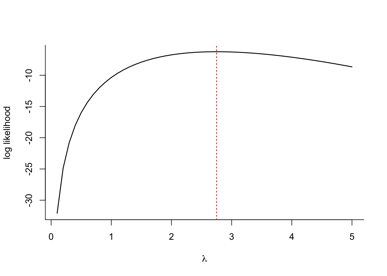
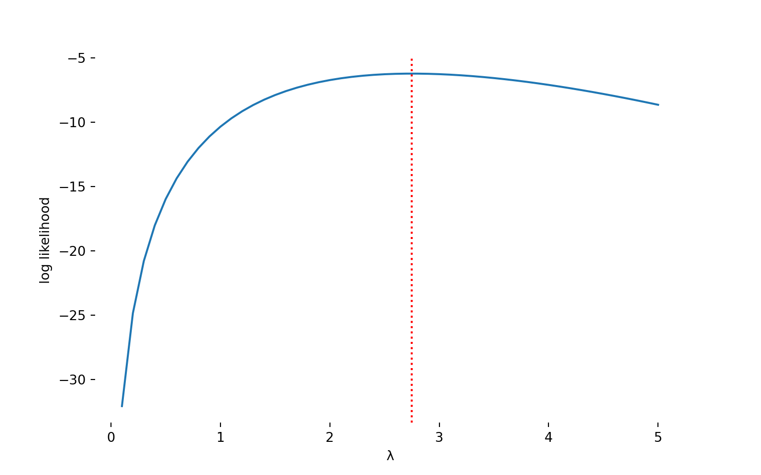
Suppose that \(n=4\) and we observe \(\textbf{y}= [3, 4, 2, 2]\). The sample mean is \(\overline{y} = 2.75\). The following R code computes the log-likelihood function \(\mathcal{l}(\lambda; \textbf{y})\) for different values of \(\lambda\). The log-likelihood function has a maximum at \(\overline{y} = 2.75\).

# Define the original data
y <- c(3, 4, 2, 2)
n <- length(y)
sumy <- sum(y)
sumlogfac <- sum(log(factorial(y)))

# Create a range of lambda values
lambda <- seq(0.1, 5, 0.1)

# Calculate log likelihood for each lambda
loglike <- log(lambda)*sumy - n*lambda - sumlogfac

plot(lambda,loglike,type="l",bty="l",lwd=1.5,
     xlab=expression(lambda),
     ylab="log likelihood")
abline(v=mean(y),lty="dotted",lwd=1.5,col="red")

import numpy as np
import matplotlib.pyplot as plt
import math
from scipy.special import factorial

# Define the original data
y = np.array([3, 4, 2, 2])
n = len(y)
sumy = np.sum(y)
sumlogfac = np.sum(np.log(factorial(y)))

# Create a range of lambda values
lambda_values = np.arange(0.1, 5.1, 0.1)

# Calculate log likelihood for each lambda
loglike = sumy * np.log(lambda_values) - n * lambda_values - sumlogfac

# Create the plot
plt.figure(figsize=(8, 5))
plt.plot(lambda_values, loglike, linewidth=1.5)
plt.axvline(x=np.mean(y), linestyle='dotted', linewidth=1.5, color='red')
plt.xlabel('λ')
plt.ylabel('log likelihood')
plt.box(False)

plt.show()

Example: MLE for iid Bernoulli Experiments

To find the maximum likelihood estimator of \(\pi\) in \(n\) iid Bernoulli(\(\pi\)) experiments, we need to find the value \(\widehat{\pi}\) that maximizes the log-likelihood function

\[\begin{align*} \mathcal{l}(\pi; \textbf{y}) &= \log\left(\prod_{i=1}^n \, \pi^{y_i} \, (1-\pi)^{1-y_i}\right) \\ &= \sum_{i=1}^n \, y_i\log(\pi) + (1-y_i)\log(1-\pi) \end{align*}\]

\(\mathcal{l}(\pi; \textbf{y}) = \sum_i y_i\log(\pi) + (1-y_i)\log(1-\pi)\). The derivative with respect to \(\pi\) is

\[\begin{align*} \frac{\partial \mathcal{l}(\pi; \textbf{y})}{\partial \pi} &= \frac{1}{\pi}\sum_{i=1}^n y_i - \frac{1}{1-\pi}\sum_{i=1}^n(1-y_i) \\ &= \frac{1}{\pi} n\overline{y} - \frac{1}{1-\pi}(n - n\overline{y}) \end{align*}\]

Setting the derivative to zero and rearranging terms we get

\[\begin{align*} \frac{1-\widehat{\pi}}{\widehat{\pi}} &= \frac{n-n\overline{y}}{n\overline{y}} \\ \frac{1}{\widehat{\pi}} &= \frac{n - n\overline{y}}{n\overline{y}} + 1 \\ \widehat{\pi} &= \overline{y} \end{align*}\]

The MLE of \(\pi\) is the sample mean.

Maximum likelihood estimation is popular because it is an intuitive principle if we accept a random data-generating mechanism. MLEs have very appealing properties, for example, they are invariant estimators. If \(\widehat{\theta}\) is the MLE of \(\theta\), then \(g(\widehat{\theta})\) is the maximum likelihood estimator of \(g(\theta)\).

Example: MLEs of Confidence Intervals

In generalized linear models, a linear predictor is related to a transformation of the mean through the link function \[ g(\mu) = \eta = \beta_0 + \beta_1x_1 + \cdots + \beta_p x_p \] For example, if the data are Poisson random variables, \(g(\cdot)\) is typically the log function (the log link). The coefficient estimates have a linear interpretation on the logarithmic scale. Suppose \(\boldsymbol{\beta}\) is estimated by maximum likelihood and is used to construct a 95% confidence interval \([\widehat{\eta}_{.025},\widehat{\eta}_{.975}]\) for \(\eta\).

You can transform from \(\eta\) to \(\mu\) by inverting the link function, \(\mu = g^{-1}(\mu)\). Thus, \[ \left[ \exp\{\widehat{\eta}_{.025}\}, \exp\{\widehat{\eta}_{.975}\} \right] \] is a 95% confidence interval for \(\mu\).

For a finite sample size, MLEs are not necessarily optimal estimators but they have appealing properties as the sample size grows. As \(n \rightarrow \infty\), maximum likelihood estimators

  • are consistent, that means they converge in probability to the true value
  • are normally distributed
  • are efficient in that no other estimator has an asymptotically smaller mean squared error

Linear Model with Gaussian Errors

Suppose we want to find an estimator for \(\boldsymbol{\beta}\) in the linear model \(\textbf{Y}= \textbf{X}\boldsymbol{\beta}+ \boldsymbol{\epsilon}\) where the model errors follow a Gaussian distribution with mean \(\textbf{0}\) and variance \(\textbf{V}\). \(\textbf{Y}\) then follows a Gaussian distribution because it is a linear function of \(\boldsymbol{\epsilon}\) (see Section 3.7). The probability density function of \(\textbf{Y}\) is

\[ f\left( \textbf{Y}\right)=\frac{\left| \textbf{V}\right|^{- 1/2}}{(2\pi)^{\frac{n}{2}}}\exp\left\{ - \frac{1}{2}\left( \textbf{Y}- \textbf{X}\boldsymbol{\beta}\right)^\prime\textbf{V}^{- 1}\left( \textbf{Y}- \textbf{X}\boldsymbol{\beta}\right) \right\} \]

This joint distribution of the data can be used to derive the maximum likelihood estimator (MLE) of \(\boldsymbol{\beta}\). Maximum likelihood estimation considers this as a function of \(\boldsymbol{\beta}\) rather than a function of \(\textbf{Y}.\) Maximizing this likelihood function \(\mathcal{l}(\boldsymbol{\beta};\textbf{Y})\) is equivalent to maximizing its logarithm. The log-likelihood function for this problem is given by

\[ \log\mathcal{l}\left( \boldsymbol{\beta};\textbf{Y}\right\} = l\left( \boldsymbol{\beta};\textbf{Y}\right) = - \frac{1}{2}\log\left( \left| \textbf{V}\right| \right) - \frac{n}{2}\log(2\pi) - \frac{1}{2}\left( \textbf{Y}- \textbf{X}\boldsymbol{\beta}\right)^\prime\textbf{V}^{- 1}\left( \textbf{Y}- \textbf{X}\boldsymbol{\beta}\right) \]

Finding the maximum of this function with respect to \(\boldsymbol{\beta}\) is equivalent to minimizing the quadratic form \[ \left( \textbf{Y}- \textbf{X}\boldsymbol{\beta}\right)^\prime\textbf{V}^{-1}\left( \textbf{Y}- \textbf{X}\boldsymbol{\beta}\right) \] with respect to \(\boldsymbol{\beta}\). Applying the results about matrix differentiation in Section 3.5 leads to

\[\begin{align*} \frac{\partial}{\partial\boldsymbol{\beta}}\left( \textbf{Y}- \textbf{X}\boldsymbol{\beta}\right)^\prime\textbf{V}^{- 1}\left( \textbf{Y}- \textbf{X}\boldsymbol{\beta}\right) &= \frac{\partial}{\partial\boldsymbol{\beta}}\left\{ \textbf{Y}^\prime\textbf{V}^{- 1}\textbf{Y}- 2\textbf{Y}^\prime\textbf{V}^{- 1}\textbf{X}\boldsymbol{\beta}+ \boldsymbol{\beta}^\prime\textbf{X}^\prime\textbf{V}^{- 1}\textbf{X}\boldsymbol{\beta}\right\} \\ &= - 2\textbf{X}^\prime\textbf{V}^{- 1}\textbf{Y}+ 2\textbf{X}^\prime\textbf{V}^{- 1}\textbf{X}\boldsymbol{\beta} \end{align*}\]

The derivative is zero when \(\textbf{X}^\prime\textbf{V}^{- 1}\textbf{Y}= \textbf{X}^\prime\textbf{V}^{- 1}\textbf{X}\boldsymbol{\beta}\).

If \(\textbf{X}\) is of full column rank, then \(\textbf{X}^\prime\textbf{V}^{- 1}\textbf{X}\) is non-singular and its inverse exists. Pre-multiplying both sides of the equation with that inverse yields the solution

\[\begin{align*} \textbf{X}^\prime\textbf{V}^{- 1}\textbf{Y}&= \textbf{X}^\prime\textbf{V}^{- 1}\textbf{X}\widehat{\boldsymbol{\beta}} \\ \left( \textbf{X}^{\prime}\textbf{V}^{- 1}\textbf{X}\right)^{- 1}\textbf{X}^\prime\textbf{V}^{- 1}\textbf{Y}&= {\left( \textbf{X}^{\prime}\textbf{V}^{- 1}\textbf{X}\right)^{- 1}\textbf{X}}^\prime\textbf{V}^{- 1}\textbf{X}\widehat{\boldsymbol{\beta}} \\ \left( \textbf{X}^{\prime}\textbf{V}^{- 1}\textbf{X}\right)^{- 1}\textbf{X}^\prime\textbf{V}^{- 1}\textbf{Y}&= \widehat{\boldsymbol{\beta}} \end{align*}\]

The maximum likelihood estimator of \(\boldsymbol{\beta}\) is the generalized least squares estimator

\[\widehat{\boldsymbol{\beta}}_{GLS} = \left( \textbf{X}^{\prime}\textbf{V}^{- 1}\textbf{X}\right)^{- 1}\textbf{X}^\prime\textbf{V}^{- 1}\textbf{Y}\]

A special case arises when the model errors \(\boldsymbol{\epsilon}\) are uncorrelated and the variance matrix \(\textbf{V}\) is a diagonal matrix:

\[ \textbf{V}= \begin{bmatrix} \sigma_{1}^{2} & \cdots & 0 \\ \vdots & \ddots & \vdots \\ 0 & \cdots & \sigma_{n}^{2} \end{bmatrix} \]

Since the errors are Gaussian distributed, we know that the errors are then independent. The MLE of \(\boldsymbol{\beta}\) is the weighted least squares estimator

\[ \widehat{\boldsymbol{\beta}}_{WLS} = \left(\textbf{X}^\prime\textbf{W}\textbf{X}\right)^{-1}\textbf{X}^\prime\textbf{W}\textbf{Y} \] where \(\textbf{W}= \textbf{V}^{-1}\).

A further special case arises when the diagonal entries are all the same,

\[\textbf{V}= \begin{bmatrix} \sigma^{2}\ & \cdots & 0 \\ \vdots & \ddots & \vdots \\ 0 & \cdots & \sigma^{2} \end{bmatrix} = \sigma^{2}\textbf{I}\]

We can write the error distribution in this case as \(\boldsymbol{\epsilon}\sim G\left(\textbf{0},\sigma^{2}\textbf{I}\right)\) and the model for \(\textbf{Y}\) as \(\textbf{Y}\sim G\left( \textbf{X}\boldsymbol{\beta},\sigma^{2}\textbf{I}\right)\).

Under this iid assumption for the Gaussian linear model we can substitute \(\sigma^{2}\textbf{I}\) for \(\textbf{V}\) in the formula for \(\widehat{\boldsymbol{\beta}}\). The maximum likelihood estimator for \(\boldsymbol{\beta}\) is the ordinary least squares estimator:

\[\widehat{\boldsymbol{\beta}}_{OLS} = \left( \textbf{X}^{\prime}\textbf{X}\right)^{- 1}\textbf{X}^\prime\textbf{Y}\]

Notice that \(\sigma^{2}\) cancels out of the formula; the value of the OLS estimator does not depend on the inherent variability of the data. However, the variability of the OLS estimator does depend on \(\sigma^{2}\) (and on \(\textbf{X}\)).

Now that we have found the MLE of \(\boldsymbol{\beta}\), the parameters in the mean function, we can also derive the MLE of the parameters in the variance-covariance structure of the multi-variate Gaussian. Let’s do this for the iid case, \(\boldsymbol{\epsilon}\sim G(\textbf{0},\sigma^2\textbf{I})\). The joint density of the data can then be written as \[ f(\textbf{Y}) = \prod_{i=1}^n (2 \pi\sigma^2)^{-1/2} \exp\left\{-\frac{1}{2\sigma^2} (y_i - \textbf{x}_i^\prime\boldsymbol{\beta})^2\right\} \] Taking logs and arranging terms, the log-likelihood function for \(\sigma^2\) is \[ \mathcal{l}(\sigma^2; \textbf{y}) = -\frac{n}{2}\log(2\pi\sigma^2) -\frac{1}{2\sigma^2}\sum_{i=1}^n(y_i - \textbf{x}_i\prime\boldsymbol{\beta})^2 \]

Taking the derivative of \(\mathcal{l}(\sigma^2; \textbf{y})\) with respect to \(\sigma^2\), setting it to zero and arranging terms results in \[ \frac{1}{\sigma^4}\sum_{i=1}^n(y_i - \textbf{x}_i^\prime\boldsymbol{\beta})^2 = \frac{n}{\sigma^2} \] The MLE of \(\sigma^2\) in this case is \[ \widehat{\sigma}^2 = \frac{1}{n}\sum_{i=1}^n(y_i - \textbf{x}_i^\prime\boldsymbol{\beta})^2 \] The MLE of \(\sigma^2\) looks similar to the estimator we used in the OLS case, \[ \frac{1}{n-r(\textbf{X})} \sum_{i=1}^n(y_i - \textbf{x}_i^\prime \widehat{\boldsymbol{\beta}})^2 = \frac{1}{n-r(\textbf{X})} \, \text{SSE} \] with two important differences. The divisor in the MLE is \(n\) instead of \(n-r(\textbf{X})\) and the MLE uses \(\boldsymbol{\beta}\) rather than the OLS estimator \(\widehat{\boldsymbol{\beta}}\) in the sum-of-squares term. In practice, we would substitute the MLE for \(\boldsymbol{\beta}\) to compute \(\widehat{\sigma}^2\), so that the least squares-based estimator and the maximum likelihood estimator differ only in the divisor. Consequently, they cannot be both unbiased estimators of \(\sigma^2\). Which should we choose?

We can think of the divisor \(n-r(\textbf{X})\) as accounting for the actual degrees of freedom, the amount of information if you will, in the estimator. Since we are using an estimate of \(\boldsymbol{\beta}\) to compute SSE, we have “used up” information in the amount of the rank of \(\textbf{X}\). This is the same rationale that computes the estimate of the sample variance as \[ s^2 = \frac{1}{n-1} \sum_{i=1}^n \left(y_i - \overline{y}\right)^2 \] because we are using the sample mean \(\overline{y}\) in the computation rather than the true mean. Once the sample mean is known, only \((n-1)\) of the \(y_i\) can be chosen freely, the value of the last one is determined.

The reason the MLE divides by \(n\) instead of \(n-r(\textbf{X})\) is that it uses \(\boldsymbol{\beta}\) and does not need to account for information already “used up” in the estimation of the mean function. If you substitute \(\widehat{\boldsymbol{\beta}}\) for \(\boldsymbol{\beta}\), the MLE of \(\sigma^2\) is a biased estimator.