We have seen in Section 12.3 that classification is based on a decision rule applied to an estimate of a probability. Any method that can predict probabilities can thus be used to classify observations. The regression approach to classification relies on such models where \(\text{E}[Y]\) is a probability (binary case) or a vector of probabilities (multinomial case). Logistic regression and multinomial regression can be used for predicting the mean response—a probability (vector)—or class membership.
13.1 Binary Data
With binary data we can apply logistic regression to predict events (positives) and non-events (negatives). Recall from Chapter 10 that a logistic regression model (with logit link) is a generalized linear model where \[
\begin{align*}
Y &\sim \text{Bernoulli}(\pi) \\
\pi &= \frac{1}{1+\exp\{-\eta\}} \\
\eta &= \textbf{x}^\prime \boldsymbol{\beta}
\end{align*}
\]
Once \(\boldsymbol{\beta}\) is estimated by maximum likelihood, predicted values on the link scale and on the mean scale are obtained as \[
\begin{align*}
\widehat{\eta} &= \textbf{x}^\prime\widehat{\boldsymbol{\beta}} \\
\widehat{\pi} &= \frac{1}{1+\exp\{-\widehat{\eta}\}}
\end{align*}
\]
and an observation is classified as an event if \(\widehat{\pi} > c\). If the threshold \(c=0.5\), the Bayes classifier results.
Example: Credit Default–ISLR
We continue the analysis of the credit default data from Chapter 10, but with the goal to classify the observations in the test data set as defaulting/not defaulting on their credit and analyzing the performance of the model based on confusion matrix, ROC and Precision-recall curves.
Recall that the Default data is part of the ISLR2 library (James et al. 2021), a simulated data set with ten thousand observations. The target variable is default, whether a customer defaulted on their credit card debt. Input variables include a factor that indicates student status, account balance and income information.
As previously, we randomly split the data into 9,000 training observations and 1,000 test observations
library(ISLR2)head(Default)
  default student   balance    income
1      No      No  729.5265 44361.625
2      No     Yes  817.1804 12106.135
3      No      No 1073.5492 31767.139
4      No      No  529.2506 35704.494
5      No      No  785.6559 38463.496
6      No     Yes  919.5885  7491.559
Call:
glm(formula = default ~ ., family = binomial, data = train)

Coefficients:
              Estimate Std. Error z value Pr(>|z|)
(Intercept) -1.106e+01  5.252e-01 -21.060   <2e-16 ***
studentYes  -6.098e-01  2.530e-01  -2.410    0.016 *
balance      5.811e-03  2.491e-04  23.323   <2e-16 ***
income       5.038e-06  8.731e-06   0.577    0.564
---
Signif. codes:  0 '***' 0.001 '**' 0.01 '*' 0.05 '.' 0.1 ' ' 1

(Dispersion parameter for binomial family taken to be 1)

    Null deviance: 2617.1  on 8999  degrees of freedom
Residual deviance: 1398.0  on 8996  degrees of freedom
AIC: 1406

Number of Fisher Scoring iterations: 8
Student status and account balance are significant predictors of credit default, the income seems less important given the other predictors (\(p\)-value of 0.5639).
The confusion matrix can be computed with the confusionMatrix function in the caret package. The option positive="Yes" identifies the level of the factor considered the “positive” level for the calculation of the statistics. This will not affect the overall confusion matrix but will affect the interpretation of sensitivity, specificity and other statistics. By default, the function uses the first level of a factor as the “positive” result which would be “No” in our case.
Before calling confusionMatrix we first calculate the predicted probabilities from the logistic regression model, then calculate the Bayes classifier (\(c=0.5\)). mode="everything" requests statistics based on sensitivity and specificity as well as statistics based on precision and recall.
Confusion Matrix and Statistics

          Reference
Prediction  No Yes
       No  958  26
       Yes   7   9

               Accuracy : 0.967
                 95% CI : (0.954, 0.9772)
    No Information Rate : 0.965
    P-Value [Acc > NIR] : 0.407906

                  Kappa : 0.3384

 Mcnemar's Test P-Value : 0.001728

            Sensitivity : 0.2571
            Specificity : 0.9927
         Pos Pred Value : 0.5625
         Neg Pred Value : 0.9736
              Precision : 0.5625
                 Recall : 0.2571
                     F1 : 0.3529
             Prevalence : 0.0350
         Detection Rate : 0.0090
   Detection Prevalence : 0.0160
      Balanced Accuracy : 0.6249

       'Positive' Class : Yes
The accuracy of the model appears high with 96.7%, but the no-information rate of 0.965 shows that the inclusion of the three input variables did not improve the model much. If you were to simply classify all observations as “No”, this naïve approach would result in an accuracy of 96.5%, simply because defaults are very rare.
The sensitivity of the model is dismal with 0.2571, the false negative rate is high (1-0.2571 = 0.7429). If someone defaults, the model has only a 25.71% chance to detect that. Not surprisingly, the specificity is very high, 958/(958+7) = 0.9927. This is again driven by the high number of non-defaulters and a low false positive rate (FPR = 7 / (958 + 7) = 0.0073).
Would changing the threshold improve the model by increasing its sensitivity? If we declare a default if the predicted probability exceeds 0.25, we get more positive predictions. How does this affect accuracy and other measures?
Confusion Matrix and Statistics

          Reference
Prediction  No Yes
       No  935  15
       Yes  30  20

               Accuracy : 0.955
                 95% CI : (0.9402, 0.967)
    No Information Rate : 0.965
    P-Value [Acc > NIR] : 0.96033

                  Kappa : 0.4479

 Mcnemar's Test P-Value : 0.03689

            Sensitivity : 0.5714
            Specificity : 0.9689
         Pos Pred Value : 0.4000
         Neg Pred Value : 0.9842
              Precision : 0.4000
                 Recall : 0.5714
                     F1 : 0.4706
             Prevalence : 0.0350
         Detection Rate : 0.0200
   Detection Prevalence : 0.0500
      Balanced Accuracy : 0.7702

       'Positive' Class : Yes
The sensitivity of the model increases, as expected, while the specificity does not take much of a hit. Interestingly, the accuracy of this decision rule has now sunk below the no-information rate. Precision has gone down but the \(F_1\) score has gone up. This decision rule balances better between precision and recall than the Bayes classifier.
The next code blocks uses the ROCR package to compute the ROC curve (Figure 13.1), the AUC, the Precision-recall curve (Figure 13.2) and the AUC-PR. The first step in using ROCR is to call the prediction function to create a prediction object. The performance function of the package is then used to compute statistics and visualizations based on that object.
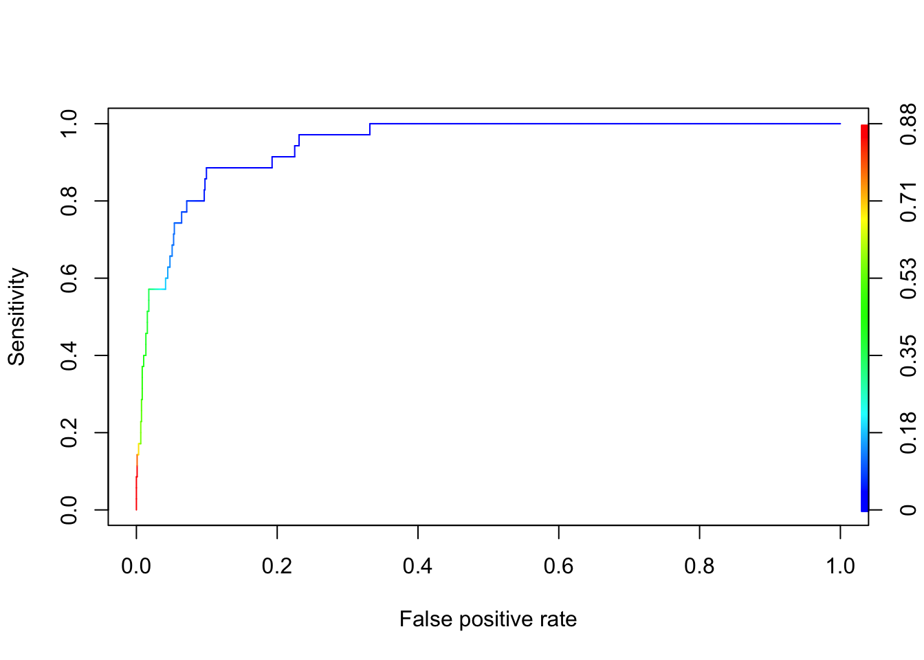
Figure 13.1: ROC curve for credit default logistic regression.
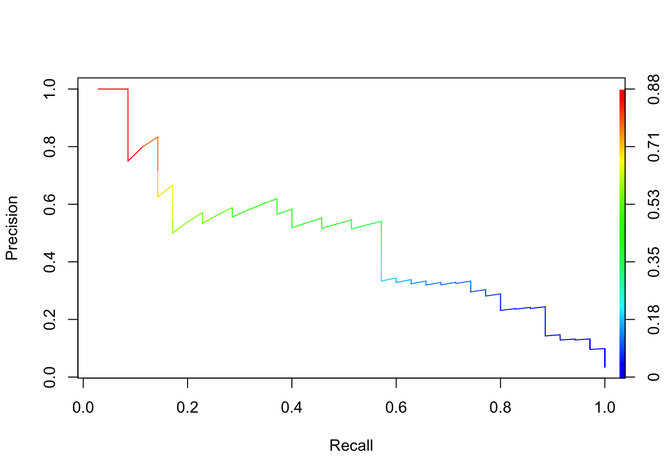
The ROC curve looks quite good for this data–model combination. The cutoffs \(c\) corresponding to the steps in the plot are shown with different colors. As the cutoff drops below 0.35, the sensitivity of the decision rule increases sharply. The area under the curve of 0.9468 is impressive. However, we know that the data are highly unbalanced, so let’s take a look at the precision-recall plot (Figure 13.2)
Figure 13.2: Precision-recall curve for credit default logistic regression.
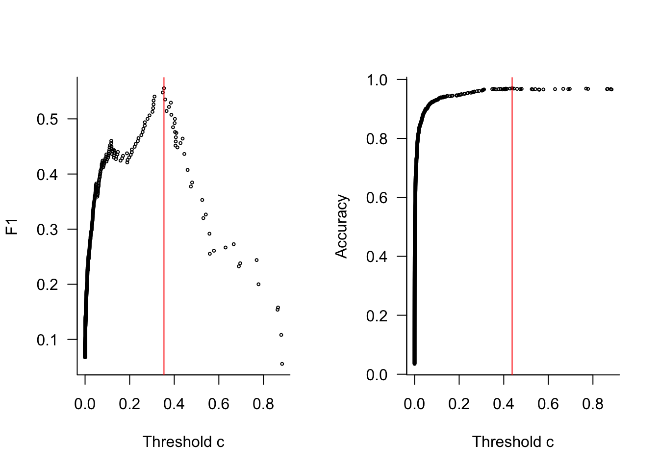
Another powerful feature of ROCR is the calculation of any measure as a function of the threshold value. The next code block computes and displays accuracy and \(F_1\) measure as a function of \(c\). Both are maximized for values in the neighborhood of \(c=0.4\)
f1 <-performance(pred_obj,"f")acc <-performance(pred_obj,"acc")par(mfrow=c(1,2))plot(f1@x.values[[1]],f1@y.values[[1]],cex=0.4,xlab="Threshold c",ylab="F1",las=1,bty="l")maxval <-which.max(f1@y.values[[1]])abline(v=f1@x.values[[1]][maxval],col="red")plot(acc@x.values[[1]],acc@y.values[[1]],cex=0.4,xlab="Threshold c",ylab="Accuracy",las=1,bty="l")maxval <-which.max(acc@y.values[[1]])abline(v=acc@x.values[[1]][maxval],col="red")
13.2 Multinomial Data
Suppose you draw \(n\) observations from a population where labels \(C_1, \cdots, C_k\) occur with probabilities \(\pi_1, \cdots, \pi_k\). The probability to observe \(C_1\) exactly \(y_1\) times, \(C_2\) exactly \(y_2\) times, and so forth, is \[
\begin{align*}
\Pr(\textbf{Y}= [y_1,\cdots,y_k]) &= \frac{n!}{y_1!y_2!\cdots y_k!} \pi_1 \times \cdots \pi_k \\
&= \frac{n!}{\prod_{j=1}^ky_j} \prod_{j=1}^k \pi_j
\end{align*}
\] This is the probability mass function of the multinomial distribution. For \(k=2\) this reduces to the binomial distribution, \[
{n \choose y} \pi^y (1-\pi)^{n-y}
\] The mean of the multinomial distribution is \(n\) times the vector of the category probabilities \(\boldsymbol{\pi} = [\pi_1, \cdots,\pi_k]^\prime\).
A classification model for multinomial data can thus be based on a multinomial regression model that predicts the category probabilities, and then applies a classification rule in a second step to determine the predicted category. How these regression models are constructed differs depending on whether the categories of the multinomial are unordered (nominal) or ordered.
Modeling Nominal Data
The models for unordered multinomial data are a direct extension of the logistic regression type models for binary data. The predicted probabilities in the logistic model are \[
\begin{align*}
\Pr(Y=1 | \textbf{x}) &= \frac{1}{1+\exp\{-\textbf{x}^\prime\boldsymbol{\beta}\}} \\
\Pr(Y=0 | \textbf{x}) &= \frac{\exp\{-\textbf{x}^\prime\boldsymbol{\beta}\}}{1+\exp\{-\textbf{x}^\prime\boldsymbol{\beta}\}}
\end{align*}
\]
Softmax function and reference category
The generalization to \(k\) categories is \[
\Pr(Y=j | \textbf{x}) = \frac{\exp\{\textbf{x}^\prime\boldsymbol{\beta}_j\}}{\sum_{l=1}^k \exp\{\textbf{x}^\prime\boldsymbol{\beta}_l\}}
\tag{13.1}\]
Each of the \(k\) categories has its own parameter vector \(\boldsymbol{\beta}_j\). But wait, why does the logistic regression model with \(k=2\) have only one (\(k-1\)) parameter vector? Since the category probabilities sum to 1, one of the probabilities is redundant, it can be calculated from the other probabilities. In multinomial logistic regression this constraint is built into the calculations by setting \(\boldsymbol{\beta}_j = \textbf{0}\) for one of the categories. This is called the reference category. Suppose we choose the first category as reference. Then Equation 13.1 becomes
\[
\begin{align*}
\Pr(Y=1 | \textbf{x}) &= \frac{1}{1 + \sum_{l=2}^k \exp\{\textbf{x}^\prime\boldsymbol{\beta}_l\}} \\
\Pr(Y=j > 1 | \textbf{x}) &= \frac{\exp\{\textbf{x}^\prime\boldsymbol{\beta}_j\}}{1 + \sum_{l=2}^k \exp\{\textbf{x}^\prime\boldsymbol{\beta}_l\}}
\end{align*}
\] If the last category is chosen as the reference, Equation 13.1 becomes \[
\begin{align*}
\Pr(Y=j < k | \textbf{x}) &= \frac{\exp\{\textbf{x}^\prime\boldsymbol{\beta}_j\}}{1 + \sum_{l=1}^{k-1} \exp\{\textbf{x}^\prime\boldsymbol{\beta}_l\}}\\
\Pr(Y=k | \textbf{x}) &= \frac{1}{1 + \sum_{l=1}^{k-1} \exp\{\textbf{x}^\prime\boldsymbol{\beta}_l\}}
\end{align*}
\]
Tip
When using software to model multinomial data, make sure to check how the code handles the reference category. There is no consistency across software packages, the choice is arbitrary. By default, SAS uses the last category as the reference, the nnet:mulitnom function in R uses the first category. The interpretation of the regression coefficients depends on the choice of the reference category. Fortunately, the predicted category probabilities do not depend on the choice of the reference category.
In addition, check on how the levels of the target variable are ordered.
In training neural networks, Equation 13.1 is called the softmax activation function (see Chapter 32). Activation functions have two important roles in neural networks: to introduce nonlinearity and to map between input and output of a network layer. The softmax activation function is used in networks that are built to classify data into \(k\) categories. Since neural networks are typically overparameterized, that is, they have more parameters than observations, the softmax transformation is applied there without constraining one of the parameter vectors to zero. This parallel development will lead us down the path in Section 35.2.3.3 to express multinomial regression for classification as a special case of a neural network (without hidden layers) and a softmax output activation.
Softmax in neural nets
Using the softmax criterion in multinomial logistic regression is the equivalence of the inverse logit link function in logistic regression. It maps from the linear predictor space to the mean of the target. The result is a probability. In neural networks, there are no distributional assumptions, so the softmax transformation should be seen as mapping \(\textbf{x}^\prime\boldsymbol{\beta}_1, \cdots, \textbf{x}^\prime\boldsymbol{\beta}_k\) to buckets of the (0,1) interval such that \[
\sum_{j=1}^k \frac{\exp\{\textbf{x}^\prime\boldsymbol{\beta}_j\}}{\sum_{l=1}^k \exp\{\textbf{x}^\prime\boldsymbol{\beta}_l\}} = 1
\] It is a stretch to think of the terms as probabilities in that context.
Multinomial Regression in R
Multiple packages can fit multinomial regression models in R.
The nnet::multinom function uses a neural network to estimate the parameters. It uses the first category as the reference.
The mlogit::mlogit function fits multinomial models by maximum likelihood and has the ability to include random effects (a multinomial mixed model). It uses a discrete choice formulation which is popular in econometrics.
We use the nnet::multinom function here and demonstrate model fitting, prediction, and classification for a simple model using the Iris data.
Before fitting a multinomial regression model, we split the data into training and test data sets with 1/3 of the observation for testing the model. Stratified sampling via caret::CreateDataPartition is used to make sure that all species are represented in the training and test data sets with appropriate proportions.
There are three species, the first level of the factor is setosa. This will be the reference level in the multinomial regression—that is, the coefficients for the I. setosa category will be set to zero. To choose a different level as the reference level, you can rearrange the factor with relevel().
The following code fits a multinomial regression model with a single input variable (Petal.Length) and target Species. The model tries to predict the iris species from just the measured length of the flower petals.
# weights:  9 (4 variable)
initial  value 112.058453
iter  10 value 13.522921
iter  20 value 12.661974
iter  30 value 12.554082
iter  40 value 12.551329
iter  50 value 12.550885
iter  60 value 12.550774
iter  70 value 12.550401
iter  80 value 12.550267
iter  90 value 12.549892
final  value 12.549891
converged
First we need to compute the terms \(\exp\{\beta_0 + \beta_1 \text{Petal.Length}\}\) for all three species. The sum of those is the term in the denominator of Equation 13.1. The following code computes the linear predictors, the denominator and the category probabilities for that observation
# The input vector for the predictionx_data <-c(1,iris_train[35,"Petal.Length"])# The coefficient vectors for the three species b_setosa <-rep(0,2)b_versicolor <- s$coefficients[1,]b_virginica <- s$coefficients[2,]# the linear predictors for the three specieseta_setosa <- x_data%*%b_setosaeta_versicolor <- x_data%*%b_versicoloreta_virginica <- x_data%*%b_virginica# The denominator for the softmax criteriondenom <-sum(exp(eta_setosa) +exp(eta_versicolor) +exp(eta_virginica))# The category probabilitiespr_setosa <-exp(eta_setosa)/denompr_versicolor <-exp(eta_versicolor)/denompr_virginica <-exp(eta_virginica)/denomcat("Pr(setosa | 4.7) = " , round(pr_setosa,4),"\n")
Confusion Matrix and Statistics

            Reference
Prediction   setosa versicolor virginica
  setosa         16          0         0
  versicolor      0         14         0
  virginica       0          2        16

Overall Statistics

               Accuracy : 0.9583
                 95% CI : (0.8575, 0.9949)
    No Information Rate : 0.3333
    P-Value [Acc > NIR] : < 2.2e-16

                  Kappa : 0.9375

 Mcnemar's Test P-Value : NA

Statistics by Class:

                     Class: setosa Class: versicolor Class: virginica
Sensitivity                 1.0000            0.8750           1.0000
Specificity                 1.0000            1.0000           0.9375
Pos Pred Value              1.0000            1.0000           0.8889
Neg Pred Value              1.0000            0.9412           1.0000
Precision                   1.0000            1.0000           0.8889
Recall                      1.0000            0.8750           1.0000
F1                          1.0000            0.9333           0.9412
Prevalence                  0.3333            0.3333           0.3333
Detection Rate              0.3333            0.2917           0.3333
Detection Prevalence        0.3333            0.2917           0.3750
Balanced Accuracy           1.0000            0.9375           0.9688
The model classifies extremely well based on just one input, Petal.Length. 2 I. versicolor are misclassified as I. virginica, the model has an accuracy of 0.9583.
In the binary classification, confusionMatrix returns a single column of confusion statistics. When \(k > 2\), a separate column is returned for each of the factor levels, comparing that level to all other levels combined. This is called the one-versus-all approach. For example, classifying I. setosa against the other two species, the model has perfect sensitivity, specificity, and recall. Classifying I. versicolor against the other species, the model has a sensitivity of 0.875.
Modeling Ordinal Data
Ordered multinomial data has category labels that imply an ordering in a greater-lesser sense. While numeric distances between the categories are not defined, we at least know that one category is more or less than another category. Examples of ordinal data are ratings (5-star scale), assessments of severity (minor, moderate, extreme), indications of sentiment (strongly disagree, disagree, agree, strongly agree), and so forth.
Cumulative link models
A statistical model for ordinal data must preserve the ordering of the data. One method of accomplishing that is to base the model on cumulative probabilities rather than category probabilities. If \(\pi_j = \Pr(Y = j)\) is the probability that \(Y\) takes on the label associated with the \(j\)th category, then \(\gamma_j = \Pr(Y \leq j)\) is called the cumulative probability of the \(j\)th category.
To classify an observation based on the cumulative probabilities, we calculate the category probabilities \[
\begin{align*}
\pi_1 &= \gamma_1 \\
\pi_j &= \gamma_j - \gamma_{j-1} \quad \text{for } 1 < j < k\\
\pi_k &= 1 - \gamma_{k-1}
\end{align*}
\]
and then assign the class with the largest category probability.
The proportional odds model (POM) is a representative of this type of model. It is also known as a cumulative link model because the link function is applied to the cumulative probabilities. In case of a logit link, the POM is \[
\text{logit}(\gamma_j) = \log\{\frac{\gamma_j}{1-\gamma_j}\} = \eta_j = \textbf{x}^\prime\boldsymbol{\beta}_j
\]
However, in contrast to the multinomial regression model for nominal data, the linear predictors in the proportional odds model are more constrained: only the intercepts vary between the categories: \[
\eta_j = \beta_{0j} + \beta_1 x_1 + \cdots + \beta_p x_p
\] The slopes are the same for all categories.
Caution
Cumulative link models can be motivated in different ways. When formulated based on a latent variable approach —where some unobserved random variable carves out segments of its support—you end up with a linear predictor of the form \[
\eta_j = \beta_{0j} - \beta_1 x_1 - \cdots - \beta_p x_p
\] As always, check the documentation! The MASS::polr function in R uses this formulation. SAS uses a linear predictor with plus signs.
In the logistic or multinomial regression model we could reduce the number of parameters because of the built-in constraint that the categories must sum to 1. A related constraint applies to cumulative link models. The cumulative probability in the last category is known to be 1, \(\gamma_k = \Pr(Y \leq k) = 1\). Thus we do not need to estimate a separate intercept for the last category. A proportional odds model with \(p=4\) inputs and \(k=3\) target categories has \(p + k-1 = 6\) parameters.
Example: Ordinal Ratings in Completely Randomized Design
For this exercise we use the data in Table 6.13 of Schabenberger and Pierce (2001, p .350). Four treatments (A, B, C, D) were assigned in a completely randomized design with four replications. The state of the replicates of the experimental units was rated as Poor, Average, or Good on four occasions (Table 13.1). For example, on the first measurement occasion all replicates of treatment A were rated in the Poor category. At the second occasion two replicates of treatment A were in Poor condition, two replicates were in Average condition.
Table 13.1: Observed frequencies for CRD measured on 4 occasions.
Rating
A
B
C
D
Poor
4,2,4,4
4,3,4,4
0,0,0,0
1,0,0,0
Average
0,2,0,0
0,1,0,0
1,0,4,4
2,2,4,4
Good
0,0,0,0
0,0,0,0
3,4,0,0
1,2,0,0
The following code creates the data in data frame format with three columns, factor rating for the target variable, factor tx for the treatment, and a date variable for the measurement occasion.
When working with ordinal target variables, we need to make sure that the factor levels are ordered correctly.
ordinal$rating[25:35]
 [1] Poor    Poor    Poor    Poor    Poor    Poor    Average Average Average
[10] Average Average
Levels: Average Good Poor
The response levels are ordered alphabetically, which is not the order in which the data should be processed. Use the factor() function to tell R how the levels should be arranged.
 [1] Poor    Poor    Poor    Poor    Poor    Poor    Average Average Average
[10] Average Average
Levels: Poor Average Good
Another issue to watch with factors is the factor-level coding. An input factor such as tx with 4 levels will not contribute 4 parameters to a model that also contains an intercept because the \(\textbf{X}\) matrix would be singular. One of the levels is usually dropped as the reference level.
R chooses the first level. SAS, for example, chooses the last level. You can use the relevel() function to tell R which level to choose as the reference. For example, the next statement makes the level with value 4 the reference level for the tx factor.
The POM can now be fit with the MASS::polr function. The method= parameter chooses the link function for the cumulative probabilities. The value of the parameter is “logistic” rather than “logit” because polr uses the latent variable formulation for the POM. Assuming that the latent variable follows a logistic distribution leads to a cumulative link model with logit link function. Because of the latent variable genesis of the model, polr constructs a linear predictor of the form \(\eta_j = \beta_{0j} - \beta_1x_1 - \cdots - \beta_p x_p\).
Call:
polr(formula = rating ~ tx + date, data = ordinal, method = "logistic")

Coefficients:
       Value Std. Error t value
tx1  -5.7070     1.4154  -4.032
tx2  -6.5191     1.5922  -4.094
tx3   1.4468     0.8633   1.676
date -0.8773     0.3539  -2.479

Intercepts:
             Value   Std. Error t value
Poor|Average -5.6152  1.5569    -3.6066
Average|Good -0.4868  1.0022    -0.4857

Residual Deviance: 57.12394
AIC: 69.12394
The output of the summary has two sections with parameter estimates. Coefficients lists the slopes of the proportional odds model. These apply the same to all categories. Intercepts displays the intercepts \(\beta_{0j}\) for the cumulative categories. The intercept labeled Poor|Average applies to \(\eta_1\), the intercept labeled Average|Good applies to \(\eta_2\).
The coefficients labeled tx1 through tx3 do not measure the effect of the treatments. They measure the difference between the treatment and the reference level. With a t value of more than 4 in absolute value, there is strong evidence that the ratings between A and D and between B and D are significantly different. Also, it appears that the rating distribution, once adjusted for treatments, changes over time; the t value for the date is larger than 2 in absolute value. You can supplement these calculations with \(p\)-values to make these statements more statistically precise.
To calculate the probability to get at most an average rating for treatment 2 at date 3 (observation # 22), the linear predictor and the (cumulative) probability are
This are the category probabilities in contrast to the cumulative probabilities. You can see the category probabilities for all levels of the response variables as
round(pom_sum$fitted.values[22,],4)
   Poor Average    Good
 0.9717  0.0281  0.0002
Observation 22 would be classified as Poor since this has the largest predicted category probability.
You can compute predictions directly and more easily with the predict function. The type="probs" option produces the predicted category probabilities, type="class" produces the classification.
Confusion Matrix and Statistics

          Reference
Prediction Poor Average Good
   Poor      29       3    0
   Average    1      20    3
   Good       0       1    7

Overall Statistics

               Accuracy : 0.875
                 95% CI : (0.7685, 0.9445)
    No Information Rate : 0.4688
    P-Value [Acc > NIR] : 1.195e-11

                  Kappa : 0.7935

 Mcnemar's Test P-Value : NA

Statistics by Class:

                     Class: Poor Class: Average Class: Good
Sensitivity               0.9667         0.8333      0.7000
Specificity               0.9118         0.9000      0.9815
Pos Pred Value            0.9062         0.8333      0.8750
Neg Pred Value            0.9688         0.9000      0.9464
Prevalence                0.4688         0.3750      0.1562
Detection Rate            0.4531         0.3125      0.1094
Detection Prevalence      0.5000         0.3750      0.1250
Balanced Accuracy         0.9392         0.8667      0.8407
The accuracy is calculated similar to the 2 x 2 case: the ratio of the sum of the diagonal cells versus the total number: (29+20+7)/64 = 0.875.
The proportional odds model has a misclassification rate of \(MCR = 1-0.875 = 0.125\).
The Kappa statistic is a measure of the strength of the agreement of the predicted and the observed values. The more counts are concentrated on the diagonal, the stronger the agreement and the larger the Kappa statistic. Values of Kappa between 0.4 and 0.6 indicate moderate agreement, 0.6-0.8 substantial agreement, > 0.8 very strong agreement.
As in the multinomial case, the confusion statistics are calculated for each category using an one-versus-all approach. For example, the sensitivity of 0.9667 for Poor is calculated by contrasting Poor against the two other classes combined: 29 / (29 + 1) = 0.9667.
James, Gareth, Daniela Witten, Trevor Hastie, and Robert Tibshirani. 2021. An Introduction to Statistical Learning: With Applications in r, 2nd Ed. Springer. https://www.statlearning.com/.
Schabenberger, O., and Francis J. Pierce. 2001. Contemporary Statistical Models for the Plant and Soil Sciences. CRC Press, Boca Raton.