16 Regression and Classification Trees

16.1 Introduction

We decided to give decision trees its own part in the material for a number of reasons.

Decision trees can be used in regression and classification settings which could place them in both Parts II and III. Trees are different from the regression approach to classification where one fits a regression-type model first to predict category probabilities and then uses them to classify the result. With decision trees, the tree is set up from the beginning as either a regression tree or a classification tree. The remaining logic of building the tree is mostly the same, apart from differences in loss functions and how predicted values are determined.
Decision trees are among the statistical learning techniques that are easiest to explain to a non-technical audience. Trees are intrinsically interpretable, a tree diagram reveals completely how an input record is processed to arrive at a prediction or classification. This makes decision trees very popular.
Decision trees are non-parametric in the sense that they do not require a distributional assumption. Whether the target variable is uniform, gamma, Poisson, or Gaussian distributed, a tree-building algorithm works the same way. No explicit assumptions about the nature of model errors, such as equal variance, are made either.
Decision trees can be applied to many problems—since they can predict and classify—but their performance is often lacking. Trees have a number of shortcomings such as high variability, sensitivity to small changes in the data, a tendency to overfit. You are trading these against advantages such as simplicity, interpretability, and the ability to handle missing values (to some extent).
Many popular statistical learning techniques, which can perform extremely well, are based on decision trees and have been developed to overcome their shortcomings. Bagged trees, random forests, gradient boosted trees, and extreme gradient boosting are examples of such methods. To understand and appreciate these popular learning approaches, we need a basic understanding of how decision trees work.

The trees described in this chapter were introduced by Breiman et al. (1984), and are known as CART (Classification and Regression Trees). Sutton (2005) gives an excellent overview of these type of trees, and discusses bagging and boosting as well.

16.2 Partitioning \(X\)-space

The principle behind building decision trees can be visualized if we consider a problem with a target variable \(Y\) and two input variables \(X_1\) and \(X_2\). \(Y\) can be a continuous target or a classification target variable. Trees are frequently introduced with this scenario because we can visualize how observed values \(\textbf{x}= [x_1,x_2]\) translate into a prediction or classification.

The basic idea is to carve up the \([X_1,X_2]\) space into \(J\) non-overlapping regions \(R_1,\cdots, R_J\) based on training data. Each region is associated with a representative value, also determined from the training data. A new observation will fall into one of the regions, and the representative value for the region is returned as the predicted value.

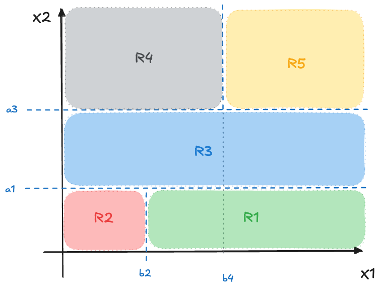
Figure 16.1: Partitioning a two-dimensional input space through binary splitting.

An example is shown in Figure 16.1. \(J=5\) regions are generated by first splitting \(X_2 \le a_1\) followed by \(X_1 \le b_2\). This creates regions \(R_1\) and \(R_2\). The next split is again applied to \(X_2\), now separating data points with \(X_2 \le a_3\). This creates region \(R_3\). The final split is splitting points where \(X_2 \ge a_3\) according to \(X_1 \le b_4\). This creates regions \(R_4\) and \(R_5\).

A display such as Figure 16.2 works for trees with \(p \le 2\) inputs. In higher dimensions we cannot visualize the regions. The typical display for a decision tree is, well, a tree. However, the tree display resembles more a root system with the trunk at the top and the branches of the tree below; or an upside down tree with the leaves at the bottom. The decision tree implied by the partitioning in Figure 16.1 is shown in Figure 16.2.

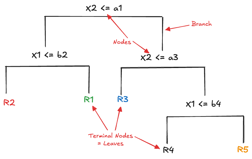
Figure 16.2: Decision tree implied by the partitioning in Figure 16.1.

The segments connecting levels of the tree are called branches, the points where the tree splits are the nodes (or internal nodes) and the end points of the tree are called the terminal nodes or the leaves. Note that having split on a variable higher up in the tree (closer to the trunk) does not preclude reusing that variable at a later point. This is evident on the right side of the tree where the tree splits on \(X_2\) a second time.

The particular form of creating the regions is called binary splitting, it leads to rectangular regions rather than irregularly shaped regions or polygons. Binary splitting is not the optimal partitioning strategy, but it leads to trees that are easy to describe and it is easier to find the regions.

Note that the coordinate system in Figure 16.1 displays \(X_1\) and \(X_2\) and not the target variable \(Y\). Where and when does the target come into the picture? The values of the target variable in the training set are used to determine

which variable to split on at any split point of the tree
the location of the splits \((a_1, b_2, \cdots)\)
the number of regions \(M\).
the representative (predicted) value in each region

In the case of a regression tree, \(Y\) is continuous and the representative value in region \(R_j\) is typically the average of the training data points that lie in \(R_j\). In the case of a classification tree, a majority vote is taken, that is, the most frequently observed category in \(R_j\) is returned as the classified value.

16.3 Training a Tree

Training a tree involves multiple steps. First, we have to decide on a criterion by which to measure the quality of a tree. For a regression tree we could consider a least-squares type residual sum of squares (RSS) criterion such as \[ \sum_{j=1}^J \sum_{i \in R_j} \left(y_i - \overline{y}_{R_j}\right)^2 \]

where \(\overline{y}_{R_j}\) is the average of the observations in the \(j\)^th region.

Once we have the criterion (the loss function) for the tree, the next step is to grow the tree until some termination criterion is met. For example, we might continue splitting nodes until all leaves contain no more than \(m\) observations. At this point we have found a tree, but not necessarily a great one. The question is how complex a tree one should build? Too many nodes and leaves with few observations and the tree will overfit and not generalize well to new observations. Too few nodes and the tree will not take advantage of the information in the training data.

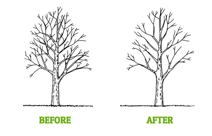
Since the predictive accuracy of trees tends to improve initially as nodes are added, the typical process is to grow the tree until a termination criterion is met and in a subsequent step to remove leaves and branches to create a smaller tree that generalizes well. Another reason for initially growing a deep tree is that a best possible split may not reduce the RSS by much, but a subsequent split can produce an appreciable decrease in RSS. By stopping too early one would miss good later splits. The process of removing nodes and branches from a deep tree is known as pruning the tree and involves a test data set or cross-validation.

Growing

Regression tree

To grow a regression tree that minimizes such a criterion we restrict the regions \(R_j\) to those obtained by recursive binary splitting as pointed out above. We first find the combination of input variable \(X_j\) and split point \(c\) such that separating the observations according to \(X_j \le c\) leads to the greatest reduction in RSS. Formally, \[ \min_{j,c} \left \{ \sum_{i:x_i \in R_1(j,c)} (y_i - \overline{y}_{R_1(j,c)})^2 + \sum_{i:x_i \in R_2(j,c)} (y_i - \overline{y}_{R_2(j,c)})^2 \right \} \] At each step of the tree-building process, we choose the pair \((j,c)\) independent of any future splits further below in the tree. In other words, we only consider the best possible split for this step, and do not look ahead. This strategy is known as a greedy algorithm.

Building the tree continues by repeating the above optimization, at each point considering the previously constructed regions instead of the entire input space. Splitting the tree continues until a termination criterion is met: for example as long as all leaves contain at least \(m\) observations.

Classification tree

A squared-error loss function works for a regression tree but not for classification problems. Besides the loss function, we also need to compute a representative value to classify observations. Let \(\widehat{p}_{jk}\) denote the proportion of training observations in region \(R_j\) that fall into class \(k\); this is simply \[ \widehat{p}_{jk} = \frac{1}{n_j}\sum_{x_i \in R_j} I(y_i = k) \] The representative value returned from region \(R_j\) is the category with the largest proportion, \(\mathop{\mathrm{arg\,max}}_k \widehat{p}_{jk}\). In other words, we take a majority vote and classify a leaf according to its most frequent category.

Based on the \(\widehat{p}_{jk}\) we can define several criteria:

Misclassification error \[ E = 1 - \max_k(\widehat{p}_{jk})\]
Gini Index \[ G = \sum_{k=1}^K \widehat{p}_{jk}(1-\widehat{p}_{jk})\]
Cross-Entropy \[ D = - \sum_{k=1}^{K} \widehat{p}_{jk} \text{log}(\widehat{p}_{jk})\]
Deviance \[ -2 \sum_{j=1}^{J} \sum_{k=1}^K n_{jk} \text{log}(\widehat{p}_{jk})\]

The misclassification error might seem as the natural criterion for classification problems, but the Gini index and the cross-entropy criterion are preferred. The misclassification error is not sensitive enough to changes in the node probabilities and is not differentiable everywhere, making it less suitable for numerical optimization.

The Gini index and cross-entropy are sensitive to node purity, leading to trees having nodes where one class dominates. To see this, consider a Bernoulli(\(\pi\)) distribution. The variance of the distribution is \(\pi(1-\pi)\) and is smallest when \(\pi \rightarrow 0\) or \(\pi \rightarrow 1\); it is highest for \(\pi= 0.5\). Nodes where \(\widehat{p}_{jk}\) is near 0 or 1 have high purity. We’d rather base classification on terminal nodes where the decision is “decisive” rather than “wishy-washy”.

Hastie, Tibshirani, and Friedman (2001, 271) give the following example of a two-category problem with 400 observations in each category. A tree with two nodes that splits observations [300,100] and [100,300] has a misclassification rate of 1/4 (200 out of 800) and a Gini index of \(2 \times 3/4 1/4 = 3/8\). A tree with nodes that splits [200,0] and [200,400] has the same misclassification rate but a lower Gini index of 2/9. The second tree would be preferred for classification.

An interesting interpretation of the Gini index is in terms of the total variance over \(K\) binary problems, each with a variance of \(\widehat{p}_{jk}(1-\widehat{p}_{jk})\). Another interpretation of the index is to imagine that rather than classifying an observation to the majority category we assign an observation to category \(k\) with probability \(\widehat{p}_{jk}\). The Gini index is the training error of this procedure.

The cross-entropy criterion also leads to nodes with higher purity than the misclassification rate. In neural networks (Chapter 32 and Chapter 33) for classification, cross-entropy is the loss function of choice.

The deviance function originates in likelihood theory and plays a greater role in pruning decision trees than in training classification trees.

Pruning

As mentioned earlier, simply applying a stop criterion based on the number of observations in the leaves (terminal nodes) does not guarantee that we have arrived at a great decision tree. Trees with many nodes and branches, also called deep trees, tend to overfit. If one were to split the tree all the way down so that each terminal leaf contains exactly one observation, the tree would be a perfect predictor on the training data.

Pruning a tree means to remove splits from a tree, creating a subtree. As subsequent splits are removed, this creates a sequence of trees, each a subtree of the previous ones.

Figure 16.3: Tree before and after pruning.

To generate a useful sequence of trees to evaluate, a process called minimum cost-complexity pruning is employed, A nested sequence of the original (full) tree is created by lopping off all nodes that emanate from a non-terminal node and the node is chosen for which a criterion such as misclassification error decreases by the smallest amount. In other words, the nodes emanating from the node are pruned that worsens the tree the least. This is known as weakest-link pruning. The performance of the subtrees is evaluated by computing a tree complexity measure based on a test data set or \(k\)-fold cross-validation.

Formally, let \(Q(T)\) be the cost criterion by which tree \(T\) is evaluated. \(Q(T)\) is RSS for a regression tree and any of the criteria listed above for classification trees (Gini index or deviance, for example). If \(|T|\) is the number of terminal nodes in \(T\), then we seek to minimize for each subtree the cost-complexity criterion \[ C_\alpha(T) = Q(T) + \alpha|T| \] where \(\alpha\) is a hyperparameter. If \(\alpha = 0\) we end up with the full tree. As \(\alpha\) increases, trees with more terminal nodes are penalized more heavily. For each value of \(\alpha\) there is one tree \(T_\alpha\) in the sequence of subtrees obtained by weakest-link pruning that minimizes \(C_\alpha(T)\).

With regression trees, the criterion used to grow the trees (squared error) is also used to prune the tree. With classification trees, growing the tree often relies on Gini index or cross-entropy, while pruning a tree uses the deviance or misclassification rate.

16.4 Issues Related to Decision Trees

Categorical Inputs

Many introductions to decision trees focus on the case where the \(X\)s are quantitative (numeric) variables. Categorical inputs (factors) can be handled easily in trees.

Suppose \(X\) is categorical with \(k\) levels in the set \(D_k\). The set of possible values can be divided into \(2^{k-1}-1\) possible partitions, which is trivial for \(k=1\) and leads to many possible partitions as \(k\) grows. However, for values of \(k > 2\), if you split the set \(D_k\) into two proper subsets \(D_s\) and \(D_l\), where \(s+l=k\), then fewer possible splits need to be considered. In other words, at each split of the categorical variable, we try to split off groups containing 1, 2, or a small number of levels from the other set.

Missing Values

It is often said that “trees can handle missing values” and by extension tree-based techniques such as random forests or gradient boosted trees are somehow robust to the presence of missing values. That is simply not true. So let us look into how missing values can be handled in decision trees.

First, observations with missing values for the target variable are not automatically handled by tree constructing software. These observation are discarded. For input variables with missing values there are two approaches.

With categorical inputs one approach is to create a new missing category. This will be considered in determining splits just like any other value of the input variable. This approach can shed light on whether observations with missing values exhibit a different pattern from complete observations. Another strategy, that applies to categorical and quantitative inputs, is the use of surrogate splits. If we come to a split in the tree and the current observation has a missing value we split on a surrogate variable that does not have missing values. In choosing surrogate variables for splits we choose variables whose splits mimic those of the primary split variable—that is, variables that are highly correlated with the primary variable. If the surrogate split variable is missing, then we can have a surrogate for the surrogate variable and so on.

Surrogate splits can be used during training and during prediction of new observations. They “handle” missingness in the sense that the observations do not need to be omitted from the analysis. However, this does not mean that the resulting analysis is OK. Unless the missing value is MCAR (missing completely at random), the analysis can be biased.

Missing Value Processes

A detailed study of missing values and their impact on statistical analysis is given in Little and Rubin (1987). They define missing value processes as MAR (missing at random) and MCAR (missing completely at random).

Suppose we collected data on inputs \(\textbf{X}\) and target \(\textbf{Y}\). Some of the rows of \(\textbf{X}\) contain missing values and \(\textbf{X}_{c}\) are the rows with complete data. Define \(\textbf{R}\) as a matrix with typical element \(r_{ij} = 1\) if the \(j\)^th input in row \(i\) is missing, and \(r_{ij} = 0\) otherwise.

The missing value process is MAR if the distribution of \(\textbf{R}\) depends on the data \(\textbf{Z}= [\textbf{Y},\textbf{X}]\) only through \(\textbf{Z}_{c} = [\textbf{Y}, \textbf{X}_c]\): \[ \Pr(\textbf{R}| \textbf{Z}) = \Pr(\textbf{R}| \textbf{Z}_{c}) \]

This essentially states that the mechanism that results in missingness is independent of the unobserved value. If furthermore the distribution of \(\textbf{R}\) does not depend on either the observed or missing data, the process is MCAR: \[ \Pr(\textbf{R}| \textbf{Z}) = \Pr(\textbf{R}) \] If a weight measurement is not taken because the scales unexpectedly malfunctioned the missing data is MAR or MCAR. If the measurement is not taken because the animal is too light or heavy for the scales, the missing value process is not MAR or MCAR. If in a longitudinal health study a patient drops out because their condition worsened, the missingness is not MAR or MCAR. We say that the missingness is informative.

An example of informative missingness is a model to predict cardiovascular risk. Because the risk is judged low, a cholesterol measurement is not taken, whereas for patients with expected higher risk for heart health such measurements are routinely done. The absence of the cholesterol measurement in electronic health records can have predictive power for a lower cardiovascular risk, its missingness is informative.

Optimality

Decision trees constructed with the CART method (or other methods) are not optimal in that they make concessions for reasons of computational expediency and interpretability.

Recursive binary splitting leads to partitions of the \(X\)-space that are simple to interpret but are not optimal partitions in terms of a loss criterion.
The greedy splitting algorithm only considers a reduction in variability or increase in purity at the current level of the tree, it does not look ahead and gauge the impact of a split on nodes further down in the tree.
Weakest-link cutting during cost-complexity pruning does not visit all subtrees, only a nested sequence of subtrees.
With large data sets, multiway splits rather than binary splits could be beneficial. We use binary splitting to prevent fragmentation of the data into small sets too quickly and hope that a subsequent split further down the tree will achieve the same as a multiway split higher up on the tree.

Stability

While decision trees are easy to interpret, the lack of stability under small changes of the data reduces their interpretability in the sense that firm conclusions based on trees are difficult. If the tree could change greatly with small changes in the data, how can we be confident that inputs that appear high in the tree (early splits) are particularly important?

On the other hand, decision trees with single splits are stable in a different sense. If single variable splits are used, the tree is invariant with respect to monotone transformations of the inputs (Sutton 2005). You do not have to worry whether to use log or square root or reciprocal transformations of an input variable in constructing the tree. As long as large values consistenly map to large transformed values or large values map consistenly to smaller values, the tree is invariant.

Smoothness

The prediction surface of decision trees is not smooth, it changes abruptly at the boundaries of the leaf nodes. In a regression application the underlying relationship \(\text{E}[Y] = f(\textbf{x})\) is normally assumed to be a smooth function of the inputs. In classification models, in particular with binary targets, this is less of an issue.

Nonlinearity and Interactions

One advantage of trees over linear model is their ability to model complex nonlinear relationships between inputs and target and non-homogeneous response. For example, the response surface can look different in some regions of the \(X\)-space compared to others. A linear model would have to use transformations and interactions to capture this in a single function across the space. A tree can easily adjust through the choice of split variables and split values in different regions of the \(X\)-space. So much so, that capturing linear relationships is actually difficult with decision trees. Hastie, Tibshirani, and Friedman (2001, 274) give the following example:

Suppose that \(Y = \beta_1 I(X_1 < t_1) + \beta_2 I(X_2 < t_2) + \epsilon\) is the underlying model. To maintain this additive relationship between \(Y\) and \([X_1,X_2]\), a tree that would first split on \(X_1\) near \(t_1\) would then have to split both nodes on \(X_2\) near \(t_2\). As Hastie, Tibshirani, and Friedman (2001) put it

…the model is given no special encouragement to find such structure. If there were ten rather than two aditive effects, … the data analyst would be hard pressed to recognize [the additive structure] in the estimated tree.

Interactions can be captured by trees. However, what appears as interaction between inputs can be caused by just correlation. Sutton (2005) gives the following example:

\(X_1\) and \(X_2\) are highly correlated inputs. A tree first splits on \(X_3\), then on \(X_1\) in the left side of the tree and on \(X_2\) in the right side of the tree. This might suggest the presence of interactions, but it could be simply that a tree split on only \(X_3\) and \(X_1\) is equivalent to one split only on \(X_3\) and \(X_2\). Both of these trees would suggest an additive relationship rather than an interaction, their equivalence stems from the correlation between \(X_1\) and \(X_2\).