12 Introduction
The target variable \(Y\) in regression is a numerical variable, either continuous or discrete (a count, for example). The regression model expresses the relationship between the expected value of \(Y\), and input variables for each of the \(i=1,\cdots,n\) samples: \[ \text{E}[Y_i | \textbf{x}_i] = f(\textbf{x}_i; \boldsymbol{\theta}) \]
12.1 Categorical Targets
In a classification problem the target variable is qualitative (categorical). The \(k\) categories of the target variable are also called the classes, hence the name classification. Recall from Section 1.2.0.4 that categorical variables belong to the discrete variables that have a countable number of values. With categorical variables, in contrast to counts, the values consist of labels, even if numbers are used for labeling.
- Multinomial Variables
Nominal variables: The labels are unordered, for example the variable “fruit” takes on the values “apple”, “peach”, “tomato” (yes, tomatoes are fruit but do not belong in fruit salad).
Ordinal variables: the category labels can be arranged in a natural order in a lesser-greater sense. Examples are 1—5 star reviews or ratings of severity (“mild”, “modest”, “severe”).
- Binary variables: take on exactly two values (dead/alive, Yes/No, 1/0, fraud/not fraud, diseased/not diseased)
The observed values of the target variable are simply labels that enumerate the possible classes. The set of labels can be as small as two, we call those binary target variables or can have thousands of elements, as can be the case when classifying objects on images or analyzing words based on a dictionary. Even if the categories are labeled numerically, we think of the numbers as identifiers for the categories, not in a numerical sense. A two-category target for customers with and without a subscription could be labeled as “subscriber”/“non-subscriber”, or “1”/“0”, or “Green”/“Blue”, and so on.
When using numeric class labels, the temptation to treat them as values of a continuous variable grows with the number of classes. A frequent example are ratings on a preference scale (Figure 12.1). If the possible ratings are 1-star, 2-stars, 3-stars, 4-stars, and 5-stars, how can we possibly achieve 0.5 or 3.5 stars?

These calculations assume that the star-scale is continuous, which implies that differences between values are defined. This is not the case. A 4-star rating is higher than a 2-star rating, but it is not double that. The distance between a 4-star and a 3-star rating is not the same as that between a 3-star and a 2-star rating. The correct way to interpret the rating scale is as an ordinal lesser-greater sense. If a website claims that a product has a rating of 4.7, they are treating the rating as continuous. The correct way to state the central tendency of the ratings is to provide estimates of the multinomial category probabilities (Figure 12.2).

Classification problems are everywhere. Here are some examples:
- Medical diagnosis: given a patient’s symptoms and history assign a medical condition
- Financial services: determine whether a payment transaction is fraudulent
- Customer intelligence: assign a new customer to a customer profile (segmentation)
- Computer vision: detect defective items on an assembly line
- Computer vision: identify objects on an image
- Text classification: detect spam email
- Digital marketing: predict which advertisement a user will click on
- Search engine: Given a user’s query and search history, predict which link they will follow
These examples show that predicting an observation and assigning an observation are ultimately the same in classification models. The predicted value in a classification model is the category we predict an observation to fall in. Depending on the type of model, this classification of an observation might first go through a prediction of another kind: the prediction of the probability of category membership. This is precisely the link between regression and classification models—more on that below.
12.2 From Label to Encoding
Separate from the labeling of the categories is the encoding of the categories. To process the data computationally, we need to replace at some point the descriptive class labels with numerical values. In logistic regression, for example, the two possible states of the target variable are coded as \(1\)s and \(0\)s where a \(1\) represents the event of interest. Another common coding scheme for the two states is to use \(1\) and \(-1\). This is common in boosting methods such as adaptive boosting (Section 21.2) and leads to a simple classification rule based on the sign of the predictor.
In situations where \(k > 2\), categories are typically one-hot encoded. This is a fancy way of saying that one \(Y\) column with \(k\) unique values is expanded into \(k\) columns \(Y_1,\cdots,Y_k\), each consists of zeros and ones. \(X_j\) contains ones in the rows where \(Y\) takes on the \(j\)th label, zero otherwise. Table 12.1 shows two categorical variables A and B with 2 and 4 levels, respectively, and their one-hot encoded expansions. A uses numerical values to identify the categories, B uses characters.
| A | \(A_1\) | \(A_2\) | B | \(B_1\) | \(B_2\) | \(B_3\) | \(B_4\) |
|---|---|---|---|---|---|---|---|
| 1 | 1 | 0 | ff | 1 | 0 | 0 | 0 |
| 1 | 1 | 0 | gg | 0 | 1 | 0 | 0 |
| 1 | 1 | 0 | hh | 0 | 0 | 1 | 0 |
| 2 | 0 | 1 | ff | 1 | 0 | 0 | 0 |
| 2 | 0 | 1 | gg | 0 | 1 | 0 | 0 |
| 2 | 0 | 1 | hh | 0 | 0 | 1 | 0 |
| 1 | 1 | 0 | ii | 0 | 0 | 0 | 1 |
There is redundant information in Table 12.1. Once you know how many categories a variable has, you can fully determine the data from \(k-1\) one-hot encoded columns. If \(Y_1,\cdots,Y_{k-1}\) are all zero, then \(Y_k = 1\); if any of the \(Y_1,\cdots,Y_{k-1}\) is \(1\), then we know that \(Y_k = 0\). In statistical models it is common to use only \(k-1\) of the encoded columns, and to treat one of the columns as a baseline. In machine learning applications using neural networks for classification it is common to use all \(k\) columns.
12.3 Classification Rule
Suppose the \(k\) possible labels of a categorical target are \(C_1, \cdots, C_k\) and the probability that \(Y_i\) takes on the label \(C_j\) is \(\Pr(Y_i=j|\textbf{x}_i)\). A classifier is a rule that assigns a predicted label based on estimates \[ \widehat{\Pr}(Y_i=j|\textbf{x}_i) \]
We use the shorthand \(Y_i\) to refer to the observed label and \(\widehat{Y}_i\) to refer to the classified value (the predicted label). So which label should we assign to \(\widehat{Y}_i\). With \(k\) classes, there are \(k\) probabilities, \(\widehat{\Pr}(Y=1|\textbf{x}), \cdots, \widehat{\Pr}(Y=k|\textbf{x})\). The most common rule is to assign the category with the highest probability. This rule is known as the Bayes classifier: \[ \widehat{Y}_i = \mathop{\mathrm{arg\,max}}_j \; \widehat{\Pr}(Y_i = j | \textbf{x}_i) \]
The Bayes classifier is optimal in the sense that no other classification rule achieves a lower misclassification rate (MCR): \[ MCR = \frac{1}{n}\sum_{i=1}^n I(\widehat{y}_i \neq y_i) \tag{12.1}\]
In Equation 12.1, \(I()\) is the identity function, returning \(1\) if the condition in parentheses is true, \(0\) otherwise. The misclassification rate is the proportion of observations for which the predicted category is different from the observed category.
In a binary problem the Bayes rule reduces to choosing the category with the largest predicted probability. Or, equivalently, predict the category coded as \(1\) if \[ \widehat{\Pr}(Y=1|\textbf{x}) > 0.5 \]
12.4 Confusion Matrix
The performance of a classification model is not measured in terms of the mean-squared error. The difference between observed and predicted category is not a meaningful measure of discrepancy. Instead, the performance of classification model is measured by comparing the (relative) frequencies of observed and predicted categories. In the binary case, the performance measures are derived from the confusion matrix of the model.
Definition: Confusion Matrix
The \(k \times k\) confusion matrix in a classification problem is the cross-classification between the observed and the predicted categories. In a problem with two categories, the confusion matrix is a \(2 \times 2\) matrix.
The cells of the matrix contain the number of data points that fall into the cross-classification when the classification rule is applied to \(n\) observations. If one of the categories is labeled positive and the other is labeled negative, the cells give the number of true positive (TP), true negative (TN), false positive (FP), and false negative (FN) predictions.
The following table shows the layout of a typical confusion matrix for a 2-category classification problem. A false positive prediction, for example, is to predict a positive (“Yes”) result when the true state (the observed state) was negative. A false negative result is when the decision rule assigns a “No” to an observation with positive state.
| Observed Category | ||
|---|---|---|
| Predicted Category | Yes (Positive) | No (Negative) |
| Yes (Positive) | True Positive (TP) | False Positive (FP) |
| No (Negative) | False Negative (FN) | True Negative (TN) |
Based on the four cells in the confusion matrix we can calculate several statistics (Table 12.2).
| Statistic | Calculation | Notes |
|---|---|---|
| False Positive Rate (FPR) | FP / (FP + TN) | The rate of the true negative cases that were predicted to be positive |
| False Negative Rate (FNR) | FN / (TP + FN) | The rate of the true positive cases that were predicted to be negative |
| Sensitivity | TP / (TP + FN) = 1 – FNR | This is the true positive rate; also called Recall |
| Specificity | TN / (FP + TN) = 1— FPR | This is the true negative rate |
| Accuracy | (TP + TN) / (TP + TN + FP + FN) | Overall proportion of correct classifications |
| Misclassification rate | (FP + FN) / (TP + TN + FP + FN) | Overall proportion of incorrect classifications, 1 – Accuracy |
| Precision | TP / (TP + FP) | Ratio of true positives to anything predicted as positive; the accuracy of positive predictions |
| \(F_1\)-score | \(\frac{2\text{Precision} \times \text{Recall}}{\text{Precision} + \text{Recall}}\) | Harmonic mean of precision and recall |
| Detection Rate | TP / (TP + TN + FP + FN) | |
| No Information Rate | \(\frac{\max(TP+FN,FP+TN)}{TP+TN+FP+FN}\) | The proportion of observations in the larger observed class |
The model accuracy is measured by the ratio of observations that were correctly classified, the sum of the diagonal cells divided by the total number of observations. The misclassification rate is the complement of the accuracy.
The sensitivity is the ratio of true positives to what should have been predicted as positive. In machine learning, this measure is called the recall of the model.
The specificity is the ratio of true negatives to what should have been predicted as negative. Sensitivity and specificity are not complements of each other; they are calculated with different denominators.
The no information rate is an interesting statistic, it represents how well a model would perform on the data if it were to assign all predictions to the more frequent class. That is the performance of a model without input variables.
Just like regression models for continuous data are often (mis-)judged based on \(R^2\), classification models are often (mis-)judged based on their accuracy. That is not without problems. The issue is that the two possible errors, false positives and false negatives, might not be of equal consequence.
Suppose a model is developed to diagnoses a serious medical condition. A false positive error is to tell a patient that they have the disease, when in fact they have not. A false negative error is the failure to diagnose the disease when the patient is ill. How to weigh the errors depends on their consequences and their prevalence.
Fraudulent credit card transactions are rare, only a fraction of a percent of all transactions are not legitimate. A false positive in a credit card fraud detection algorithm means that a legitimate transaction is flagged as fraudulent with potentially embarrassing consequences for the card holder—a declined transaction when nothing was wrong. A false negative means not detecting a fraudulent transaction—which is rare to begin with. Banks try their hardest to reduce the false positive rate of their fraud detection models, a 2% change in that rate affects many more customers than a 2% change in the false negative rate. If it turns out later that a fraudulent transaction occurred, the bank will still make its customers whole. When a bank reaches out to you to confirm a transaction they are trying to manage potential false positives.
It might not matter how accurate a model is unless it achieves a certain sensitivity—the ability to correctly identify positives.
Consider the data in the Table 12.3, representing 1,000 observations and predictions.
| Observed Category | ||
|---|---|---|
| Predicted Category | Yes (Positive) | No (Negative) |
| Yes (Positive) | 9 | 7 |
| No (Negative) | 26 | 958 |
The classification has an accuracy of 96.7%, which seems impressive. Its false positive and false negative rates are very different, however: FPR = 0.0073, FNR = 0.7429. The model is much less likely to predict a “Yes” when the true state is “No”, than it is to predict a “No” when the true state is “Yes”. Whether we can accept a model with such low sensitivity (100 – 74.29) = 25.71% is questionable, despite the high accuracy. An evaluation of this model should consider whether the two errors, false positive and false negative predictions, are of equal importance and consequence.
It is also noteworthy that the accuracy of 96.7% is not as impressive if you check the no-information rate of the data. The proportion of observations in the larger observed class is (958 + 7)/1,000 = 0.965. The accuracy of the decision rule is only slightly larger. In other words, if you were to take a naïve (dumb) approach and predict all observations as “No” without looking at the data, that naïve decision rule would have an accuracy of 96.5%. The use of input variables to improve the model has not helped much compared to a dumb model. The accuracy improved by only .2 percentage points.
Table 12.2 also lists the \(F_1\)-score, a combination of precision and recall (sensitivity) that is popular in machine learning. The \(F_1\)-score is the harmonic mean of the two basic measures: \[ \begin{align*} F_1 &= \frac{2}{\frac{1}{\text{Precision}}+\frac{1}{\text{Recall}}} \\ &= \frac{2\,\text{Precision}\times\text{Recall}}{\text{Precision} + \text{Recall}} \\ &= \frac{\frac{TP}{(TP+FP)(TP+FN)}}{\frac{1}{TP+FP} + \frac{1}{TP+FN}} \end{align*} \tag{12.2}\]
\(F_1\) is bounded \(0 \le F_1 \le 1\); a model with \(F_1 = 1\) has perfect precision and recall.
The \(F_1\)-score is sometimes preferred over accuracy when the data are unbalanced—that is, negative and positive outcomes occur with very different proportions. However, the \(F_1\) can be misleading for unbalanced cases since it does not take into account the number of true negatives (there is no TN in Equation 12.2). The \(F_1\) score is also not symmetric; if you exchange the roles of positives and negatives, you can get a different \(F_1\), the accuracy will remain the same. The \(F_1\) score can be a good performance measure for binary classification when you want a model that has both high sensitivity (high recall) and high precision. Such a model combines a low rate of false positives with a low rate of false negatives. If the costs of errors are the same, balancing recall and precision makes sense.
12.5 Receiver Operator Characteristic (ROC) and Area under the Curve (AUC)
So why do we not build models that have a high accuracy, small false positive rate, and small false negative rate? That seems desirable and we can affect those parameters through the decision rule. To reduce the likelihood of a false positive we could require more evidence before predicting a positive result. Similarly, to reduce the likelihood of false negatives, we could make it more difficult to classify an observation as negative. If \(c\) is the threshold in the decision rule of a binary classification, we could treat it as a parameter and evaluate the performance of the model for different rules
\[ \widehat{\Pr}(Y=1|\textbf{x}) > c \] You can easily see that changing \(c\) affects both false positives and false negatives, as well as the accuracy. For \(c=0.5\) you arrive at the accuracy-optimal Bayes classifier.
To see how the choice of cutoff affects the performance of a binary classifier, several graphical devices are in use. The receiver operator characteristic (ROC) is a plot of the true positive rate (TPR, sensitivity, recall) against the false positive rate for different values of \(c\). It shows the sensitivity of the classifier as a function of the false positive rate (Figure 12.3).
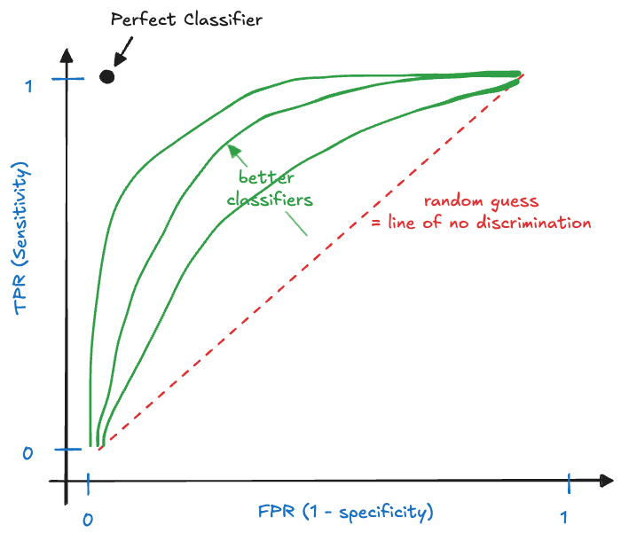
The name receiver operator characteristic stems from the method’s origin, it was developed in World War II for operators of military radar receivers to detect enemy objects in battlefields, specifically after the attack on Pearl Harbor in 1941 to measure the operator’s ability to correctly detect Japanese aircraft in radar signals.
A perfect model is one with perfect sensitivity and perfect specificity, it makes no incorrect predictions. It is represented by the point at the (0,1) coordinate in Figure 12.3. The diagonal line represents a random classifier. Suppose you are flipping a coin to predict positive outcomes. The long-run (expected) behavior of this decision rule is captured by the diagonal line. If the coin is fair, you get a point on the line at coordinate (0.5, 0.5). Loaded coins where one side is more likely than the other generate the other points on the 45-degree line.
An actual model will be somewhere between the random classifier and the perfect model. The closer the operating curve is to the left and upper margins of the plot, the more performant the model. Actual ROC curves appear as step functions, after calculating FPR and TPR for a set of threshold values \(c_1, c_2, \cdots\).
The ROC curve shows how sensitivity and specificity change with the threshold value \(c\) and help solve the tradeoff between sensitivity and specificity of the model. The ROC is often summarized by computing AUC, the area under the curve. AUC is a single summary statistic that ranges from 0 to 1, with the uninformative random classifier at AUC = 0.5. The idealistic optimal ROC line that passes through (0, 1) has an AUC of 1. While AUC is a popular summary of a binary classifier, it is not without problems:
Reducing the ROC curve to a single number hides the tradeoffs associated with choosing thresholds; that is the point of the ROC in the first place.
The integration under the ROC curve incorporates extreme ranges of FPR one would usually not consider in real applications. If a false positive rate of more than 80% is unacceptable, why consider such decision rules in evaluating the performance of a model? Typically we are interested in regions of the ROC rather than the entire curve. In screening tests interest is in the ranges of low FPR, for example. To overcome this issue, partial AUC statistics have been proposed. These restrict FPR, TPR, or both to certain regions of interest.
Many performance metrics have 0 as the point of uninformedness, for example, correlation coefficients and \(R^2\). For AUC this point is 0.5, the area under the diagonal line in Figure 12.3. If someone presents an AUC of 0.36 for their classification model, remember that it performs worse than a random coin flip.
I attended a seminar where a statistician presented a new model for classifying brain conditions. Their model slightly beat out different approaches, all of them had AUCs less than 0.5! It is embarrassing if after months or years of expenditures and time spent developing methodology, collecting data, and computing a coin flip would have been more accurate.
12.6 Precision-Recall Curve
Another graphical display that summarizes the performance of a binary classifier across multiple thresholds is the precision-recall curve (Figure 12.4). Like the ROC, it compares actual classifiers against a no-skill baseline (the horizontal line drawn at the proportion of positives) and an ideal classifier.
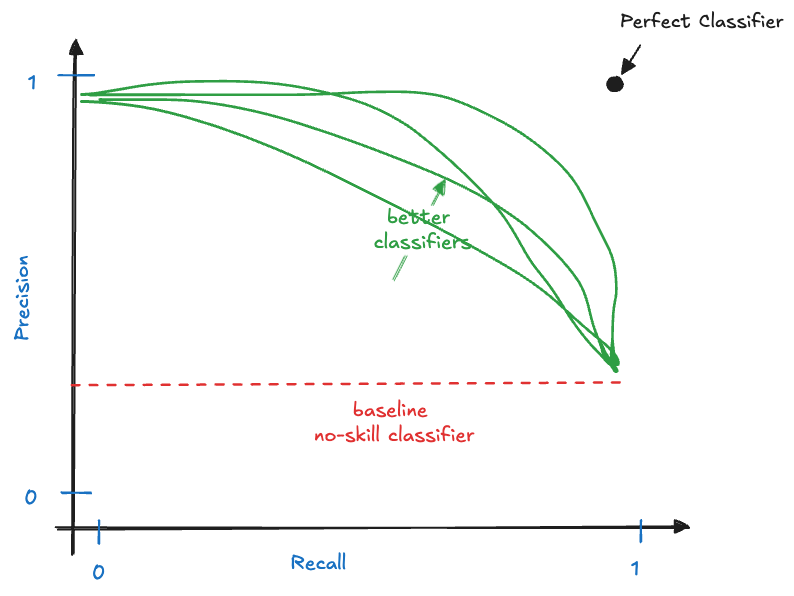
The precision-recall curve can also be summarized by computing the area under its curve (AUC-PR). A large area under the precision-recall curve indicates high precision and high recall of the model across the thresholds. Precision-recall curves are preferred over ROC curves when the data are very imbalanced with respect to positive and negative outcomes.
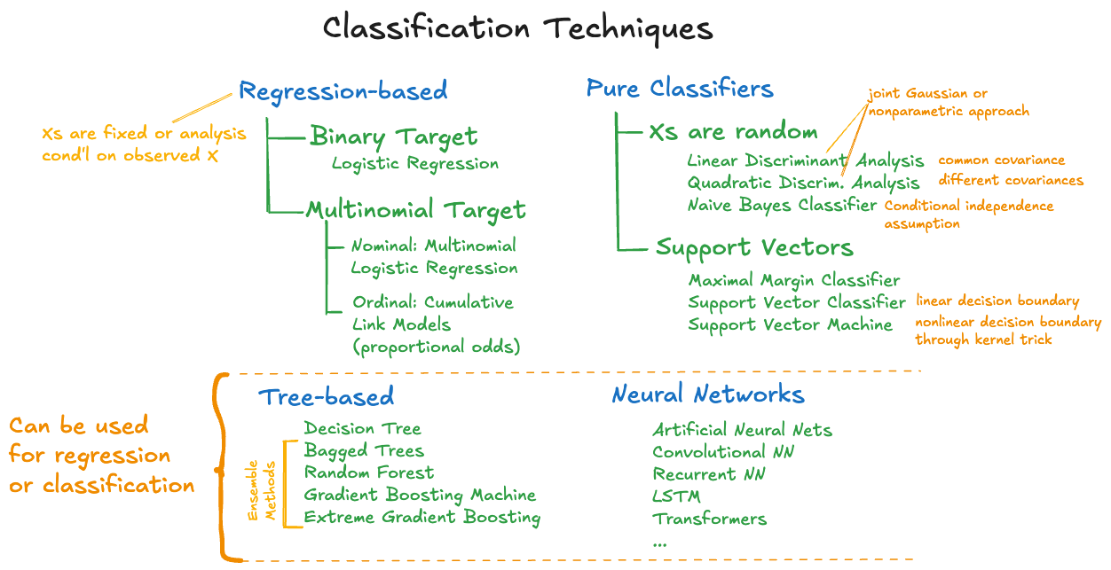
12.7 Types of Classification Models
The remaining chapters of this part are dedicated to specific types of classification models: regression-based models, pure classifiers approaches assuming the \(X\)s are random, and support vector machines. Figure 12.5 organizes these approaches. However, there are many other methods that can be used in both a regression and a classification context. For example, decision trees, boosting machines, artificial neural networks and more. These techniques are covered in other parts of the material.