library(mclust)
mb_eii <- Mclust(iris[,-5],G=3,verbose=FALSE, modelNames="EII")
mb_eii$parameters$pro
[1] 0.3333956 0.4135728 0.2530316\(K\)-means and hierarchical clustering discussed in Chapter 25 have in common that an observation is assigned to exactly one cluster; this is referred to as hard clustering. Also, the methods are nonparametric in the sense that no distributional assumptions were made. The clusters are based solely on the distance (dissimilarity) between data points. The goal of clustering is finding regions that contain modes in the distribution of \(p(\textbf{X})\). The implicit assumption of \(K\)-means and hierarchical clustering is that regions where many data points are close according to the chosen distance metric are regions where the density \(p(\textbf{X})\) is high.
In model-based clustering, this is made explicit through assumptions about the form of \(p(\textbf{X})\), the joint distribution of the variables. An important side effect of its probabilistic formulation is that observations no longer belong to just one cluster. They have a non-zero probability to belong to any cluster, a property referred to as soft clustering. An advantage of this approach lies in the possibility to assign a measure of uncertainty to cluster assignments.
A common assumption is that the distribution of \(\textbf{X}\) follows a finite mixture model (FMM), that is, it comprises a finite number \(k\) of component distributions.
In general, a finite mixture distribution is a weighted sum of \(k\) probability distributions where the weights sum to one: \[ p(Y) = \sum_{j=1}^k \pi_j \, p_j(Y) \quad \quad \sum_{j=1}^k \pi_j = 1 \] \(p_j(Y)\) is called the \(j\)th component of the mixture and \(\pi_j\) is the \(j\)th mixing probability, also referred to as the \(j\)th mixture weight. The finite mixture is called homogeneous when the \(p_j(Y)\) are of the same family, and heterogeneous when they are from different distributional families. An important example of a heterogeneous mixture, discussed in Section 10.6, is a zero-inflated model for counts, a two-component mixture of a constant distribution and a classical distribution for counts such as the Poisson or Negative Binomial.
The class of finite mixture models (FMM) is very broad and the models can get quite complicated. For example, each \(p_j(Y)\) could be a generalized linear model and its mean can depend on inputs and parameters. The mixing probabilities can also be modeled as functions of inputs and parameters using logistic (2-component models) or multinomial model types.
How do mixtures of distributions come about? An intuitive motivation is through a latent variable process. A discrete random variable \(S\) takes on states \(j=1,\cdots,k\) with probabilities \(\pi_j\). It is called a latent variable because we cannot observe it directly. We only observe its influence on the distribution of \(Y\), the variable we are interested in, and that depends on \(S\). This dependence results in a different conditional distribution of \(Y\) for each of the possible states of \(S\), \(p(Y| S=j)\). We can then derive the marginal distribution of \(Y\), the distribution we are interested in, by integrating out (summing over) \(S\) in the joint distribution
\[\begin{align*} p(Y) &= \sum_{j=1}^k \Pr(Y, S=j) \\ &= \sum_{j=1}^k \Pr(S=j) \, p(Y|S=j) = \sum_{j=1}^k \pi_j \, p_j(Y) \end{align*}\]
This is the same as computing the weighted sum over the conditional distributions–the finite mixture formulation. We cannot observe \(S\) directly, it exerts its influence on \(Y\) through the likelihood of its states (\(\pi_j\)) and the conditional distributions of \(Y|S=j\).
A special case of FMMs are Gaussian mixtures where the component distributions are multivariate Gaussian. (See Section 3.9 for a review of the multivariate Gaussian distribution.) The mixture distribution in model-based clustering is \[ p(\textbf{X}) = \sum_{j=1}^k \pi_j \, G(\boldsymbol{\mu}_j,\boldsymbol{\Sigma}_j) \]
Each \(G(bmu_j,\boldsymbol{\Sigma}_j)\) is a \(p\)-variate Gaussian, \(\boldsymbol{\mu}_j\) and \(\boldsymbol{\Sigma}_j\) are the \((p \times 1)\) mean vector and the \((p \times p)\) covariance matrix of the \(j\)th component. These need to be estimated. In terms of clusters, \(\boldsymbol{\mu}_j\) is the center of the \(j\)th cluster and \(\boldsymbol{\Sigma}_j\) determines the volume, shape, and orientation of the \(j\)th cluster.
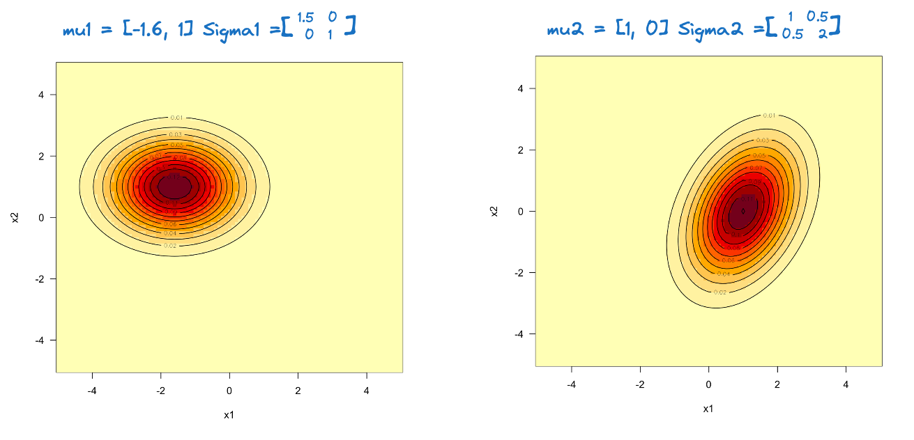
Figure 26.1 shows contours of the density for two bivariate (\(p=2\)) Gaussian distributions. The distribution on the right has \[\boldsymbol{\mu}_1 = \left [ \begin{array}{c}1 \\ 0\end{array} \right ] \qquad \boldsymbol{\Sigma}_1 = \left [ \begin{array}{cc} 1 & 0.5 \\ 0.5 & 2\\ \end{array} \right] \] and the distribution on the left has
\[\boldsymbol{\mu}_2 = \left [ \begin{array}{c}-1.6 \\ 1\end{array} \right ] \qquad \boldsymbol{\Sigma}_2 = \left [ \begin{array}{cc} 1.5 & 0 \\ 0 & 1\\ \end{array} \right] \] When the variance-covariance matrix is diagonal, the contours align with the axes of the coordinate system, stretching in the direction of greater variance. The covariance between \(X_1\) and \(X_2\) introduces a rotation of the contours in the graphic on the right.
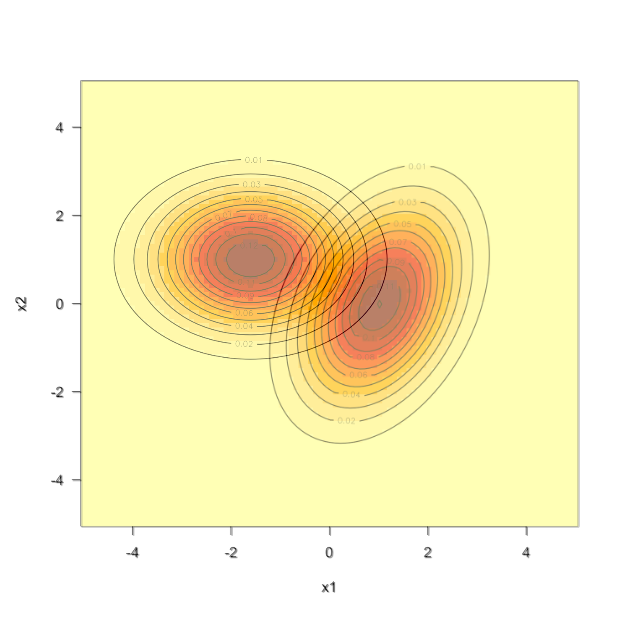
The Gaussian mixture model (GMM) can be viewed as a soft version of \(K\)-means clustering. The latter assigns an observation to exactly one of \(K\) clusters—a hard assignment. The GMM assigns probabilities of cluster membership to each observation based on \(G(\boldsymbol{\mu}_1,\boldsymbol{\Sigma}_1), \cdots, G(\boldsymbol{\mu}_k,\boldsymbol{\Sigma}_k)\). GMM allows for a “gray area”; an observation has a non-zero probability to belong to any of the \(k\) clusters (Figure 26.2).
Mclust in RRTo train a Gaussian mixture model on data in R we need to estimate the following parameters: \(k\), the number of components, \(\boldsymbol{\mu}_1, \cdots, \boldsymbol{\mu}_k\), the means of the distributions, and \(\boldsymbol{\Sigma}_1, \cdots, \boldsymbol{\Sigma}_k\), the variance-covariance matrices of the distributions (covariance matrix for short). Each \(\boldsymbol{\mu}_j\) is a \(p \times 1\) vector and each \(\boldsymbol{\Sigma}_j\) is a \(p \times p\) matrix with up to \(p(p+1)/2\) unique entries. The total number of potential unknowns in a GMM is thus \[
k \times (p + p(p+1)/2) = k\frac{3p + p^2}{2}
\]
A mixture with \(k=5\) components and \(p=10\) variables has 325 unknowns. For \(p=20\) this grows to 1,150 unknowns. That is not a large number compared to say, an artificial neural network, but it is a substantial number for estimation by maximum likelihood or Bayesian methods. To reduce the number of parameters and to add interpretability, the class of mixtures considered is constrained by imposing structure on the covariance matrices of the Gaussian distributions.
The most constrained covariance model is to assume that the variables are uncorrelated and have the same variance across the \(k\) clusters (an equal variance model): \[ \boldsymbol{\Sigma}_1 = \boldsymbol{\Sigma}_2 = \cdots = \boldsymbol{\Sigma}_k = \sigma^2 \textbf{I} \]
The next most constrained model allows for a different variance in each cluster but maintains uncorrelated inputs: \[ \boldsymbol{\Sigma}_j = \sigma^2\textbf{I} \] To capture the relevant covariance structures in model-based clustering, Fraley and Raftery (2002) start from the eigendecomposition of \(\boldsymbol{\Sigma}\) and use the general parameterization \[ \boldsymbol{\Sigma}_j = \lambda_j \textbf{D}_j \textbf{A}_j \textbf{D}_j^\prime \]
\(\textbf{D}_j\) is an orthogonal matrix of eigenvectors, \(\textbf{A}_j\) is a diagonal matrix whose elements are proportional to the eigenvalues, and \(\lambda_j\) is a proportionality constant. The highly constrained equal variance model corresponds to the special case \(\boldsymbol{\Sigma}_j = \lambda \textbf{I}\) and the heterogeneous variance model corresponds to \(\boldsymbol{\Sigma}_j = \lambda_j \textbf{I}\).
The idea behind this parameterization is to hold elements constant across clusters or vary them, and because \(\lambda\), \(\textbf{D}\), and \(\textbf{A}\) represent different aspects of the shape of the covariance matrix, one arrives at a reasonable set of possible models to consider and to compare. The geometric aspects of the component distributions captured by the three elements of the decomposition are
For example, the model \[ \boldsymbol{\Sigma}_j = \lambda \textbf{D}_j \textbf{A}\textbf{D}_j^\prime \] imposes equal volume and equal shape across the clusters, but allows for cluster-specific orientation of the distributions.
One could use other parameterizations of covariance matrices, for example, expressing covariances as functions of distance between values—the parameterization shown here is implemented in the Mclust function of the popular mclust package in R.
‘mclust’ uses a three-letter code to identify a specific covariance model (Table 26.1)
mclust.
| mclust Code | \(\boldsymbol{\Sigma}_j\) | Volume | Shape | Orientation | Notes |
|---|---|---|---|---|---|
EII |
\(\lambda \textbf{I}\) | Equal | Identity | NA | Spherical |
VII |
\(\lambda_j \textbf{I}\) | Variable | Identity | NA | Spherical |
EEI |
\(\lambda \textbf{A}\) | Equal | Equal | Coord. axes | Diagonal |
VEI |
\(\lambda_j \textbf{A}\) | Variable | Equal | Coord. axes | Diagonal |
EVI |
\(\lambda \textbf{A}_j\) | Equal | Variable | Coord. axes | Diagonal |
VVI |
\(\lambda_j \textbf{A}_j\) | Variable | Variable | Coord. axes | Diagonal |
EEE |
\(\lambda\textbf{D}\textbf{A}\textbf{D}^\prime\) | Equal | Equal | Equal | Elliptical |
EEV |
\(\lambda\textbf{D}_j \textbf{A}\textbf{D}_j^\prime\) | Equal | Equal | Variable | Elliptical |
VEV |
\(\lambda_j\textbf{D}_j \textbf{A}\textbf{D}_j^\prime\) | Variable | Equal | Variable | Elliptical |
VVV |
\(\lambda_j\textbf{D}_j \textbf{A}_j\textbf{D}_j^\prime\) | Variable | Variable | Variable | Elliptical |
The first six models in Table 26.1 have diagonal covariance matrices, the inputs are independent (lack of correlation does equal independence for Gaussian random variables). Models EEE, EEV, VEV, and VVV capture correlations among the \(X\)s and vary different aspects of \(\boldsymbol{\Sigma}_j\) across the clusters. The EEE model applies the same covariance matrix in all clusters, EEV varies orientation, VEV varies orientation and volume, and VVV varies all aspects across clusters.
The choice of covariance model should not be taken lightly, it has considerable impact on the clustering analysis. Assuming independent inputs is typically not reasonable. However, if model-based clustering is applied to the components of a PCA, this assumption is met. Some of the models in Table 26.1 are nested and can be compared through a hypothesis test. But in addition to choosing the covariance model, we also need to choose \(k\), the number of clusters. One approach is to compare the model-\(k\) combinations by way of BIC, the Bayesian information criterion, introduced in Section 22.2.1.
BIC is based on the log-likelihood, which is accessible because we have a full distributional specification, and a penalty term that protects against overfitting. Before applying model-based clustering in a full analysis to select \(k\) and the covariance models, let’s examine how to interpret the results of model-based clustering and some of the covariance structures for the Iris data.
Model-based clustering based on a finite mixture of Gaussian distributions is implemented in the Mclust function of the mclust package in R. Maximum likelihood estimates are derived by EM (Expectation-Maximization) algorithm and models are compared via BIC. An iteration of the EM algorithm comprises two steps. The E-step computes at the current estimates an \((n \times k)\) matrix \(\textbf{Z}\) of conditional probabilities that observation \(i=1,\cdots,n\) belongs to component \(j=1,\cdots,k\). The M-step updates the parameter estimates given the matrix \(\textbf{Z}\).
MclustExample: Equal Variance Structure for Iris Data
The following statements fit a 3-component mixture with EII covariance model to the numerical variables in the Iris data. The EII model is the most restrictive multivariate model, assuming diagonal covariance matrices and equal variances across variables and clusters (see Table 26.1). This model is probably not appropriate for the Iris data but simple enough to interpret the results from the analysis.
The G= and modelNames= option in Mclust are used to specify the number of components in the mixture (the number of clusters) and the covariance model. The defaults are G=1:9 and all available covariance models based on whether \(p=1\) or \(p>1\) and whether \(n > p\) or \(n \le p\).
library(mclust)
mb_eii <- Mclust(iris[,-5],G=3,verbose=FALSE, modelNames="EII")
mb_eii$parameters$pro[1] 0.3333956 0.4135728 0.2530316The three Gaussian distributions mix with probabilities \(\widehat{\pi}_1 =\) 0.3334, \(\widehat{\pi}_2 =\) 0.4136, and \(\widehat{\pi}_3 =\) 0.253.
mb_eii$parameters$mean [,1] [,2] [,3]
Sepal.Length 5.0060172 5.903268 6.848623
Sepal.Width 3.4278263 2.748010 3.074750
Petal.Length 1.4622880 4.400526 5.732651
Petal.Width 0.2461594 1.432036 2.074895The first component has a mean of \(\widehat{\boldsymbol{\mu}}_1\) = [5.006, 3.4278, 1.4623, 0.2462]. The following lists the covariance matrices in the three clusters, the model forces them to be diagonal, to have the same variance for all variables and across the clusters, \(\widehat{\lambda}_j\) = 0.1331.
mb_eii$parameters$variance$modelName
[1] "EII"
$d
[1] 4
$G
[1] 3
$sigma
, , 1
Sepal.Length Sepal.Width Petal.Length Petal.Width
Sepal.Length 0.1330939 0.0000000 0.0000000 0.0000000
Sepal.Width 0.0000000 0.1330939 0.0000000 0.0000000
Petal.Length 0.0000000 0.0000000 0.1330939 0.0000000
Petal.Width 0.0000000 0.0000000 0.0000000 0.1330939
, , 2
Sepal.Length Sepal.Width Petal.Length Petal.Width
Sepal.Length 0.1330939 0.0000000 0.0000000 0.0000000
Sepal.Width 0.0000000 0.1330939 0.0000000 0.0000000
Petal.Length 0.0000000 0.0000000 0.1330939 0.0000000
Petal.Width 0.0000000 0.0000000 0.0000000 0.1330939
, , 3
Sepal.Length Sepal.Width Petal.Length Petal.Width
Sepal.Length 0.1330939 0.0000000 0.0000000 0.0000000
Sepal.Width 0.0000000 0.1330939 0.0000000 0.0000000
Petal.Length 0.0000000 0.0000000 0.1330939 0.0000000
Petal.Width 0.0000000 0.0000000 0.0000000 0.1330939
$Sigma
Sepal.Length Sepal.Width Petal.Length Petal.Width
Sepal.Length 0.1330939 0.0000000 0.0000000 0.0000000
Sepal.Width 0.0000000 0.1330939 0.0000000 0.0000000
Petal.Length 0.0000000 0.0000000 0.1330939 0.0000000
Petal.Width 0.0000000 0.0000000 0.0000000 0.1330939
$sigmasq
[1] 0.1330939
$scale
[1] 0.1330939Based on the underlying \(\textbf{Z}\) matrix of the EM algorithm at convergence, the observations can be classified based on the highest probability.
For observation #53, for example, \(\textbf{z}_{53}\) = [0, 0.3068, 0.6932]. The probability is highest that the observation belongs to the third component, hence its cluster membership is classified as 3.
round(mb_eii$z[53,],4)[1] 0.0000 0.3068 0.6932mb_eii$classification[53][1] 3One of the big advantages of model-based clustering is the ability to quantify the uncertainty associated with a cluster assignment. How confident are we in assigning observation #53 to cluster 3? We are certain that it does not belong to cluster 1, but there is a non-zero probability that the observation belongs to cluster 2. You can retrieve the uncertainty associated with the classification of each observation in the uncertainty vector. For observations 50—55, for example:
round(mb_eii$uncertainty[50:55],4)[1] 0.0000 0.3289 0.0015 0.3068 0.0000 0.0031There is no uncertainty associated with classifying #50. An examination of \(\textbf{z}_{50}\) shows that \(z_{50,1} = 1.0\). There is uncertainty associated with the next three observations, and it is higher for #51 and #53 than for #52.
The uncertainty is simply the complement of the highest component probability. For #53, this is 1-0.6932 = 0.3068. The following code validates this for all observations.
c <- apply(mb_eii$z,1,which.max)
probs <- rep(0,length(c))
for (i in seq_along(c)) {probs[i] <- mb_eii$z[i,c[i]]}
sum(mb_eii$uncertainty - (1-probs))
[1] 0Finally, you can plot the classification, uncertainty, and density contours for the analysis by choosing the what= parameter of the plot method.
plot(mb_eii, what="classification")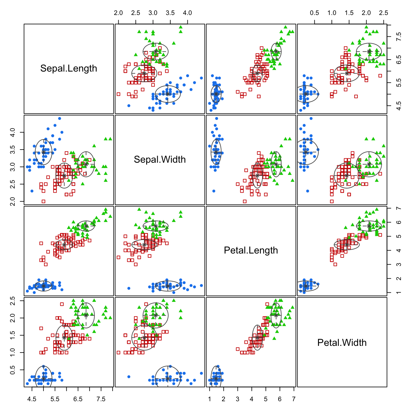
plot(mb_eii, what="uncertainty",dimens=c(1,2))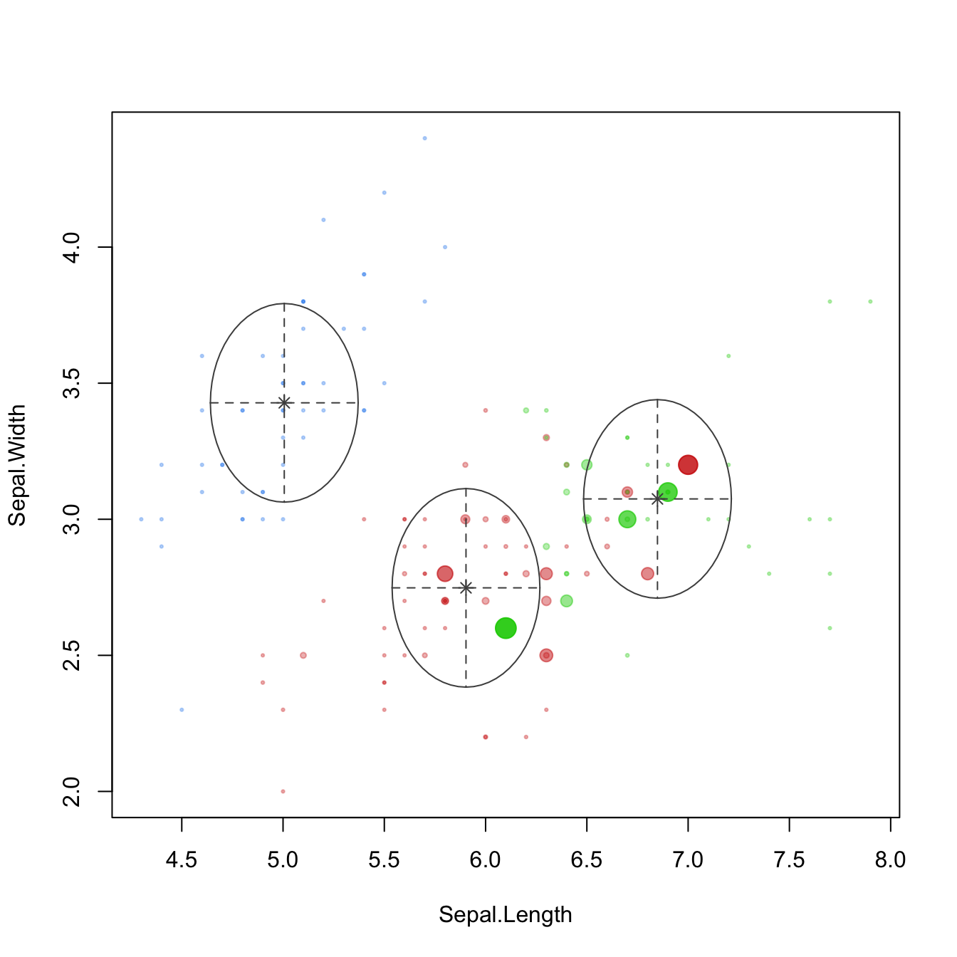
plot(mb_eii, what="density")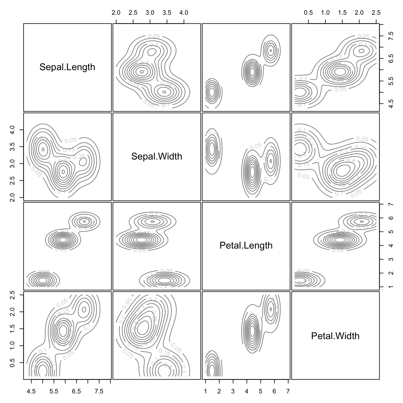
The classification and uncertainty plots are overlaid with the densities of the components. The parallel alignment of the densities with the coordinate axes reflects the absence of correlations among the variables. The volume of the densities does not capture the variability of most attributes, many points fall outside of the density contour—the equal variance assumption across variables and clusters is not justified.
Example: Other Covariance Structures for Iris Data
Now let’s look at how the choice of covariance structure affects the results of the cluster analysis. The following statements fit 3-component models with four additional covariance structures:
mb_vii <- Mclust(iris[,-5],G=3,verbose=FALSE, modelNames="VII")
mb_vei <- Mclust(iris[,-5],G=3,verbose=FALSE, modelNames="VEI")
mb_eee <- Mclust(iris[,-5],G=3,verbose=FALSE, modelNames="EEE")
mb_vev <- Mclust(iris[,-5],G=3,verbose=FALSE, modelNames="VEV")

mb_vii$parameters$variance$sigma
, , 1
Sepal.Length Sepal.Width Petal.Length Petal.Width
Sepal.Length 0.075755 0.000000 0.000000 0.000000
Sepal.Width 0.000000 0.075755 0.000000 0.000000
Petal.Length 0.000000 0.000000 0.075755 0.000000
Petal.Width 0.000000 0.000000 0.000000 0.075755
, , 2
Sepal.Length Sepal.Width Petal.Length Petal.Width
Sepal.Length 0.1629047 0.0000000 0.0000000 0.0000000
Sepal.Width 0.0000000 0.1629047 0.0000000 0.0000000
Petal.Length 0.0000000 0.0000000 0.1629047 0.0000000
Petal.Width 0.0000000 0.0000000 0.0000000 0.1629047
, , 3
Sepal.Length Sepal.Width Petal.Length Petal.Width
Sepal.Length 0.1635866 0.0000000 0.0000000 0.0000000
Sepal.Width 0.0000000 0.1635866 0.0000000 0.0000000
Petal.Length 0.0000000 0.0000000 0.1635866 0.0000000
Petal.Width 0.0000000 0.0000000 0.0000000 0.1635866mb_vii$bic[1] -853.8144For the VII model, the covariance matrices are uncorrelated and the variances of the inputs are the same. Compared to the EII model of the previous run, the variances now differ across the clusters.
Note that mclust computes the BIC statistic in a “larger-is-better” form—see the note in Section 22.2.1 on the two versions of the BIC criterion.
mb_vei$parameters$variance$sigma, , 1
Sepal.Length Sepal.Width Petal.Length Petal.Width
Sepal.Length 0.1190231 0.00000000 0.0000000 0.0000000
Sepal.Width 0.0000000 0.07153324 0.0000000 0.0000000
Petal.Length 0.0000000 0.00000000 0.0803479 0.0000000
Petal.Width 0.0000000 0.00000000 0.0000000 0.0169908
, , 2
Sepal.Length Sepal.Width Petal.Length Petal.Width
Sepal.Length 0.2655657 0.0000000 0.0000000 0.00000000
Sepal.Width 0.0000000 0.1596058 0.0000000 0.00000000
Petal.Length 0.0000000 0.0000000 0.1792731 0.00000000
Petal.Width 0.0000000 0.0000000 0.0000000 0.03791006
, , 3
Sepal.Length Sepal.Width Petal.Length Petal.Width
Sepal.Length 0.3380558 0.0000000 0.0000000 0.00000000
Sepal.Width 0.0000000 0.2031725 0.0000000 0.00000000
Petal.Length 0.0000000 0.0000000 0.2282084 0.00000000
Petal.Width 0.0000000 0.0000000 0.0000000 0.04825817mb_vei$bic[1] -779.1566The VEI model introduces different variances for the attributes and has a larger (better) BIC than the VEI model.
mb_eee$parameters$variance$sigma, , 1
Sepal.Length Sepal.Width Petal.Length Petal.Width
Sepal.Length 0.26392812 0.08980761 0.16970269 0.03931039
Sepal.Width 0.08980761 0.11191917 0.05105566 0.02992418
Petal.Length 0.16970269 0.05105566 0.18674400 0.04198254
Petal.Width 0.03931039 0.02992418 0.04198254 0.03965846
, , 2
Sepal.Length Sepal.Width Petal.Length Petal.Width
Sepal.Length 0.26392812 0.08980761 0.16970269 0.03931039
Sepal.Width 0.08980761 0.11191917 0.05105566 0.02992418
Petal.Length 0.16970269 0.05105566 0.18674400 0.04198254
Petal.Width 0.03931039 0.02992418 0.04198254 0.03965846
, , 3
Sepal.Length Sepal.Width Petal.Length Petal.Width
Sepal.Length 0.26392812 0.08980761 0.16970269 0.03931039
Sepal.Width 0.08980761 0.11191917 0.05105566 0.02992418
Petal.Length 0.16970269 0.05105566 0.18674400 0.04198254
Petal.Width 0.03931039 0.02992418 0.04198254 0.03965846mb_eee$bic[1] -632.9647The EEE model introduced covariances between the inputs but keeps the covariance matrices constant across clusters. Its BIC value of -632.965 is a further improvement over that of the VEI model.
mb_vev$parameters$variance$sigma, , 1
Sepal.Length Sepal.Width Petal.Length Petal.Width
Sepal.Length 0.13320850 0.10938369 0.019191764 0.011585649
Sepal.Width 0.10938369 0.15495369 0.012096999 0.010010130
Petal.Length 0.01919176 0.01209700 0.028275400 0.005818274
Petal.Width 0.01158565 0.01001013 0.005818274 0.010695632
, , 2
Sepal.Length Sepal.Width Petal.Length Petal.Width
Sepal.Length 0.22572159 0.07613348 0.14689934 0.04335826
Sepal.Width 0.07613348 0.08024338 0.07372331 0.03435893
Petal.Length 0.14689934 0.07372331 0.16613979 0.04953078
Petal.Width 0.04335826 0.03435893 0.04953078 0.03338619
, , 3
Sepal.Length Sepal.Width Petal.Length Petal.Width
Sepal.Length 0.42943106 0.10784274 0.33452389 0.06538369
Sepal.Width 0.10784274 0.11596343 0.08905176 0.06134034
Petal.Length 0.33452389 0.08905176 0.36422115 0.08706895
Petal.Width 0.06538369 0.06134034 0.08706895 0.08663823mb_vev$bic[1] -562.5522The VEV model allows for correlated attributes and varies volume and orientation across clusters, keeping the shape of the densities the same. Its BIC value of -562.552 indicates a further improvement over the previous models.
The choice of covariance structures and the number of mixture components can be combined into a single analysis.
Example: Selecting Structure and Number of Components
To obtain a full analysis of relevant covariance structures for \(1 \le k \le 9\), simply do not specify the G= or modelNames= arguments. Alternatively, you can limit the number of combinations considered by specifying vectors for these options.
mbc <- Mclust(iris[,-5],verbose=FALSE)
summary(mbc)
----------------------------------------------------
Gaussian finite mixture model fitted by EM algorithm
----------------------------------------------------
Mclust VEV (ellipsoidal, equal shape) model with 2 components:
log-likelihood n df BIC ICL
-215.726 150 26 -561.7285 -561.7289
Clustering table:
1 2
50 100 Based on \(9 \times 10 = 90\) models considered, Mclust choose the VEV structure with \(k=2\) mixture components. Its BIC value is -561.7285. You can see the BIC values of all 90 models and a list of the top three models in the BIC object:
mbc$BICBayesian Information Criterion (BIC):
EII VII EEI VEI EVI VVI EEE
1 -1804.0854 -1804.0854 -1522.1202 -1522.1202 -1522.1202 -1522.1202 -829.9782
2 -1123.4117 -1012.2352 -1042.9679 -956.2823 -1007.3082 -857.5515 -688.0972
3 -878.7650 -853.8144 -813.0504 -779.1566 -797.8342 -744.6382 -632.9647
4 -893.6140 -812.6048 -827.4036 -748.4529 -837.5452 -751.0198 -646.0258
5 -782.6441 -742.6083 -741.9185 -688.3463 -766.8158 -711.4502 -604.8131
6 -715.7136 -705.7811 -693.7908 -676.1697 -774.0673 -707.2901 -609.8543
7 -731.8821 -698.5413 -713.1823 -680.7377 -813.5220 -766.6500 -632.4947
8 -725.0805 -701.4806 -691.4133 -679.4640 -740.4068 -764.1969 -639.2640
9 -694.5205 -700.0276 -696.2607 -702.0143 -767.8044 -755.8290 -653.0878
VEE EVE VVE EEV VEV EVV VVV
1 -829.9782 -829.9782 -829.9782 -829.9782 -829.9782 -829.9782 -829.9782
2 -656.3270 -657.2263 -605.1841 -644.5997 -561.7285 -658.3306 -574.0178
3 -605.3982 -666.5491 -636.4259 -644.7810 -562.5522 -656.0359 -580.8396
4 -604.8371 -705.5435 -639.7078 -699.8684 -602.0104 -725.2925 -630.6000
5 NA -723.7199 -632.2056 -652.2959 -634.2890 NA -676.6061
6 -609.5584 -661.9497 -664.8224 -664.4537 -679.5116 NA -754.7938
7 NA -699.5102 -690.6108 -709.9530 -704.7699 -809.8276 -806.9277
8 -654.8237 -700.4277 -709.9392 -735.4463 -712.8788 -831.7520 -830.6373
9 NA -729.6651 -734.2997 -758.9348 -748.8237 -882.4391 -883.6931
Top 3 models based on the BIC criterion:
VEV,2 VEV,3 VVV,2
-561.7285 -562.5522 -574.0178 Model-\(k\) combinations shown as NA failed to converge based on the default settings of the EM algorithm; these can be tweaked with the control= option of Mclust. The BIC of the winning combination is
max(na.omit(apply(mbc$BIC,1,max)))[1] -561.7285which.max(na.omit(apply(mbc$BIC,1,max)))2
2 The plot of the BIC values shows two distinct groups of models (Figure 26.3). The models with diagonal covariance structure generally have lower (worse) BIC values if \(k < 6\). The difference between \(k=2\) and \(k=3\) is generally small for the models with correlations. [VEV, \(k=3\)] is a close competitor to the overall “best” model, [VEV, \(k=2\)]. Since we know that there are three species in the data set one might be tempted to go with \(k=3\). In fact, it seems that the \(k=2\) model separates I. setosa in one cluster from the other two species (Figure 26.4).
plot(mbc, what="BIC")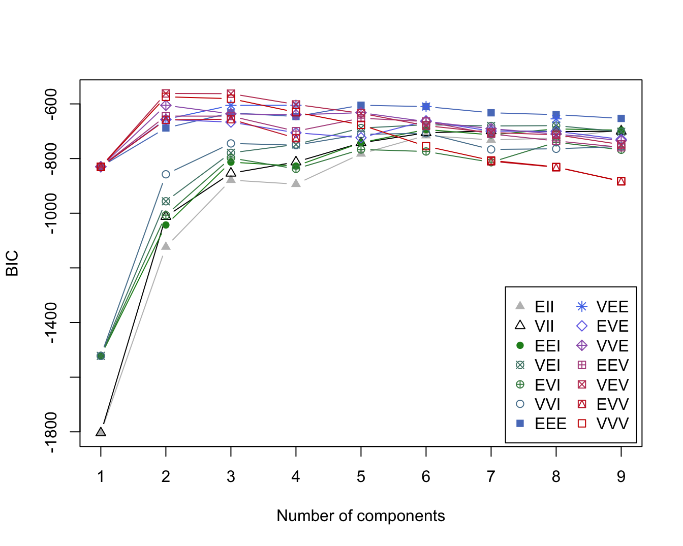
plot(mbc, what="classification",cex=0.75)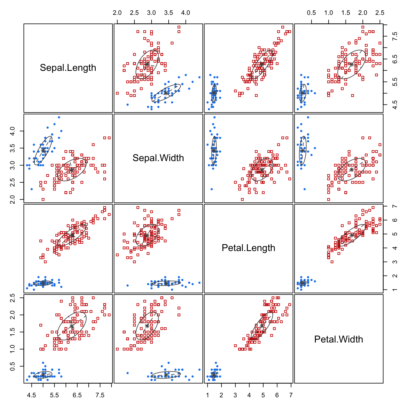
GaussianMixture in PythonPythonPython class GaussianMixture offers a simpler but more limited parameterization than the R mclust package. The covariance structure is controlled by the covariance_type parameter with four options that represent different constraints on the covariance matrices across components:
The geometric interpretation of these covariance types is:
GaussianMixture.
covariance_type |
Volume | Shape | Orientation | Notes |
|---|---|---|---|---|
spherical |
Variable | Identity | NA | Spherical |
diag |
Variable | Variable | Coord. axes | Diagonal |
tied |
Equal | Equal | Equal | Elliptical |
full |
Variable | Variable | Variable | Elliptical |
The first two models (spherical and diag) have diagonal covariance matrices, meaning the input features are independent within each component. The tied and full models can capture correlations among the features.
The choice of covariance model should not be taken lightly, it has considerable impact on the clustering analysis. Assuming independent inputs is typically not reasonable. However, if model-based clustering is applied to the components of a PCA, this assumption is met. The covariance types represent nested models that can be compared using BIC, Bayesian information criteria. But in addition to choosing the covariance model, we also need to choose \(k\), the number of clusters. One approach is to compare the model-\(k\) combinations by way of BIC introduced in Section 22.2.1.
BIC, computed with the .bic() function, is based on the log-likelihood, which is accessible because we have a full distributional specification, and a penalty term that protects against overfitting. Before applying model-based clustering in a full analysis to select \(k\) and the covariance models, let’s examine how to interpret the results of model-based clustering and some of the covariance structures for the Iris data.
GaussianMixtureExample: Spherical Structure for Iris Data
The n_components= and covariance_type= options in GaussianMixture are used to specify the number of components in the mixture (the number of clusters) and the covariance model. The defaults are n_components=1 and covariance_type='full', each component having its own general covariance matrix.
import duckdb
from sklearn.mixture import GaussianMixture
from sklearn.covariance import EmpiricalCovariance

con = duckdb.connect(database="ads.ddb", read_only=True)
iris = con.sql("SELECT * FROM iris;").df()
con.close()

iris_features = iris.drop(columns=iris.columns[-1])

#Fit the model
mb_spherical = GaussianMixture(n_components=3, covariance_type='spherical', random_state=42)
mb_spherical.fit(iris_features)
GaussianMixture(covariance_type='spherical', n_components=3, random_state=42)In a Jupyter environment, please rerun this cell to show the HTML representation or trust the notebook.
GaussianMixture(covariance_type='spherical', n_components=3, random_state=42)
# Get parameters
print(f"Mixing proportions: {mb_spherical.weights_}")
Mixing proportions: [0.25549114 0.33333333 0.41117552]The three Gaussian distributions mix with probabilities \(\widehat{\pi}_1 = 0.2555\), \(\widehat{\pi}_2 = 0.3333\), and \(\widehat{\pi}_3 = 0.4112\).
import pandas as pd
import numpy as np

print(f"\nMeans:\n {round(pd.DataFrame(mb_spherical.means_, columns=iris_features.columns).T, 4)}")
Means:
                    0      1       2
Sepal.Length  6.8419  5.006  5.9017
Sepal.Width   3.0718  3.428  2.7479
Petal.Length  5.7229  1.462  4.3984
Petal.Width   2.0705  0.246  1.4309
The first component has a mean of \(\widehat{\boldsymbol{\mu}}_1\) = [6.8419, 3.0718, 5.7229, 2.0705]. The following lists the variances in each of the three clusters, the model forces each component to have its own single variance, \(\widehat{\lambda}_j\) = [0.1644, 0.0758, 0.162].
print(f"\nVariances (spherical):\n {mb_spherical.covariances_}")
Variances (spherical):
[0.1644286 0.075756 0.16244304]For observation #53, for example, \(\textbf{z}_{53}\) = [0.663, 0, 0.337]. The probability is highest that the observation belongs to the third component, hence its cluster membership is classified as 0.
posterior_probs_53 = pd.DataFrame(mb_spherical.predict_proba(iris_features)[52], index = [0,1,2])
print(f"\nPosterior probabilities for 53rd observation:\n {np.round(posterior_probs_53.T, 4)}")
Posterior probabilities for 53rd observation:
        0    1      2
0  0.663  0.0  0.337
classifications = mb_spherical.predict(iris_features)
print(f"\nClassification for 53rd observation: {classifications[52]}")
Classification for 53rd observation: 0One of the big advantages of model-based clustering is the ability to quantify the uncertainty associated with a cluster assignment. How confident are we in assigning observation #53 to cluster 0? We are certain that it does not belong to cluster 1, but there is a non-zero probability that the observation belongs to cluster 2. You can calculate the uncertainty associated with the classification of each observation from the output of .predict_proba function. For observations 50—55, for example:
posterior_probs = mb_spherical.predict_proba(iris_features)

# Calculate uncertainty (1 - max posterior probability)
max_probs = np.max(posterior_probs, axis=1)
uncertainty = 1 - max_probs
print(f"\nUncertainty for observations 50-55 (0-indexed as 49-54):\n{np.round(uncertainty[49:55], 4)}")
Uncertainty for observations 50-55 (0-indexed as 49-54):
[0.     0.3659 0.0053 0.337  0.     0.0094]
There is no uncertainty associated with classifying #50. An examination of \(\textbf{z}_{50}\) shows that \(z_{50,1} = 1.0\). There is uncertainty associated with the next three observations, and it is higher for #51 and #53 than for #52.
The uncertainty is simply the complement of the highest component probability.
Python does not have the same plotting function capabilities as R. However, below is an example for creating a density plot with Sepal Length and Petal Length.
#Create the model with only Sepal Length and Petal Length
sep_len_pet_len_spherical = GaussianMixture(n_components=3, covariance_type='spherical', random_state=42)
sep_len_pet_len_spherical.fit(iris_features[['Sepal.Length', 'Petal.Length']])
GaussianMixture(covariance_type='spherical', n_components=3, random_state=42)In a Jupyter environment, please rerun this cell to show the HTML representation or trust the notebook.
GaussianMixture(covariance_type='spherical', n_components=3, random_state=42)
import matplotlib.pyplot as plt
from matplotlib.colors import LogNorm
import seaborn as sns

plt.figure(figsize=(8, 6))
x = np.linspace(2.0, 9.0)
y = np.linspace(0.0, 8.0)
X, Y = np.meshgrid(x, y)
XX = np.array([X.ravel(), Y.ravel()]).T
Z = -sep_len_pet_len_spherical.score_samples(XX)
Z = Z.reshape(X.shape)


sns.scatterplot(data=iris, x='Sepal.Length', y='Petal.Length', hue='Species')
#plt.scatter(iris_features['Sepal.Length'], iris_features['Petal.Length'], 5)

CS = plt.contour( X, Y, Z, norm=LogNorm(vmin=0.01, vmax=1.0), levels=np.logspace(0, 1, 10), colors = 'gray', linewidths=1 )

plt.title("GMM Contour Density Plot, Petal Length vs. Sepal Length")
plt.axis("tight")
(2.0, 9.0, 0.0, 8.0)plt.show() 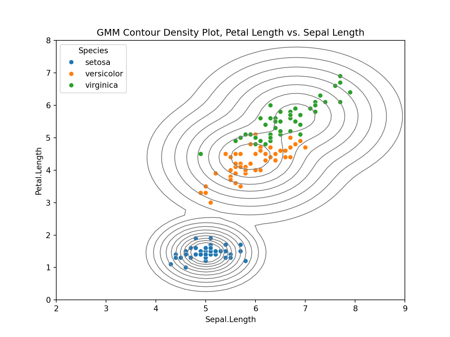
Example: Other Covariance Structures for Iris Data
Now let’s look at how the choice of covariance structure affects the results of the cluster analysis. The following statements fit 3-component models with the remaining three covariance structures:
mb_diag = GaussianMixture(n_components=3, covariance_type='diag', random_state=42)
mb_diag.fit(iris_features)
GaussianMixture(covariance_type='diag', n_components=3, random_state=42)In a Jupyter environment, please rerun this cell to show the HTML representation or trust the notebook.
GaussianMixture(covariance_type='diag', n_components=3, random_state=42)
mb_tied = GaussianMixture(n_components=3, covariance_type='tied', random_state=42)
mb_tied.fit(iris_features)
GaussianMixture(covariance_type='tied', n_components=3, random_state=42)In a Jupyter environment, please rerun this cell to show the HTML representation or trust the notebook.
GaussianMixture(covariance_type='tied', n_components=3, random_state=42)
mb_full = GaussianMixture(n_components=3, covariance_type='full', random_state=42)
mb_full.fit(iris_features)
GaussianMixture(n_components=3, random_state=42)In a Jupyter environment, please rerun this cell to show the HTML representation or trust the notebook.
GaussianMixture(n_components=3, random_state=42)
mb_spherical.bic(iris_features)853.8235771916477The BIC for the previous spherical model, which required a single variance per component, is 853.82.
Note that .bic() computes the BIC statistic in a “smaller-is-better” form—see the note in Section 22.2.1 on the two versions of the BIC criterion.
print(f"\nVariances (diagonal):\n {mb_diag.covariances_}")
Variances (diagonal):
  [[0.28520059 0.08200975 0.25128562 0.06109484]
 [0.121765   0.140817   0.029557   0.010885  ]
[0.23145596 0.08738014 0.27563102 0.0688713 ]]mb_diag.bic(iris_features)744.6403610652327The diag model introduces different variances for the attributes and a smaller (better) BIC than the spherical model.
print(f"\nVariances (tied):\n {mb_tied.covariances_}")
Variances (tied):
  [[0.2633317  0.08760867 0.1731573  0.0374331 ]
 [0.08760867 0.11040074 0.04836891 0.02701142]
 [0.1731573  0.04836891 0.20285285 0.04347376]
[0.0374331 0.02701142 0.04347376 0.03619053]]mb_tied.bic(iris_features)633.8462467337689The tied model introduces covariances between the inputs but keeps the covariance matrices constant across the clusters. Its BIC value of 633.85 is an improvement over the diag model.
print(f"\nVariances (full):\n {mb_full.covariances_}\n")
Variances (full):
  [[[0.38744093 0.09223276 0.30244302 0.06087397]
  [0.09223276 0.11040914 0.08385112 0.05574334]
  [0.30244302 0.08385112 0.32589574 0.07276776]
  [0.06087397 0.05574334 0.07276776 0.08484505]]

 [[0.121765   0.097232   0.016028   0.010124  ]
  [0.097232   0.140817   0.011464   0.009112  ]
  [0.016028   0.011464   0.029557   0.005948  ]
  [0.010124   0.009112   0.005948   0.010885  ]]

 [[0.2755171  0.09662295 0.18547072 0.05478901]
  [0.09662295 0.09255152 0.09103431 0.04299899]
  [0.18547072 0.09103431 0.20235849 0.06171383]
[0.05478901 0.04299899 0.06171383 0.03233775]]]mb_full.bic(iris_features)580.8612784697606The full model allows for correlated attributes and varied volume and shape across clusters. Its BIC value of 580.86 indicates a further improvement over the previous models.
The choice of covariance structures and the number of mixture components can be combined into a single analysis.
Example: Selecting Structure and Number of Components
To obtain a full analysis of relevant covariance structures, you can create a loop for all of the combinations to be considered.
# Test different numbers of components and covariance types
n_components_range = range(1, 10)  # Test 1-9 components
covariance_types = ['spherical', 'diag', 'tied', 'full']

bic_results = {}
all_models = {}
bic_matrix = np.full((len(n_components_range), len(covariance_types)), np.nan)

for i, n_comp in enumerate(n_components_range):
    for j, cov_type in enumerate(covariance_types):
        try:
            model = GaussianMixture(n_components=n_comp, covariance_type=cov_type,
                                  random_state=42, max_iter=200)
            model.fit(iris_features)
            bic = model.bic(iris_features)

            key = f"{cov_type}_{n_comp}"
            bic_results[key] = bic
            all_models[key] = model
            bic_matrix[i, j] = bic

        except Exception as e:
            # Some models might not converge
            bic_matrix[i, j] = np.nan
GaussianMixture(max_iter=200, n_components=9, random_state=42)In a Jupyter environment, please rerun this cell to show the HTML representation or trust the notebook.
GaussianMixture(max_iter=200, n_components=9, random_state=42)
# Find best model (lowest BIC)
valid_bics = [(k, v) for k, v in bic_results.items() if not np.isnan(v)]
best_model_key = min(valid_bics, key=lambda x: x[1])[0]
best_bic = bic_results[best_model_key]
mbc = all_models[best_model_key]

def mbc_sum (best_model_key, best_bic, mbc):

  print(f"\nBest model: {best_model_key}")
  print(f"Best BIC: {best_bic:.2f}")

  # Summary equivalent to summary(mbc) in R
  print(f"\nMODEL SUMMARY:")
  print("-" * 40)
  print(f"Model: Gaussian Mixture Model")
  print(f"Number of components: {mbc.n_components}")
  print(f"Covariance type: {mbc.covariance_type}")
  print(f"BIC: {best_bic:.2f}")
  print(f"Log-likelihood: {mbc.score(iris_features) * len(iris_features):.2f}")
  print(f"Number of parameters: {mbc._n_parameters()}")
mbc_sum (best_model_key, best_bic, mbc)
Best model: full_2
Best BIC: 574.02

MODEL SUMMARY:
----------------------------------------
Model: Gaussian Mixture Model
Number of components: 2
Covariance type: full
BIC: 574.02
Log-likelihood: -214.35
Number of parameters: 29
You can create a dataframe to view the BIC results from all of the models.
# Create BIC DataFrame for better visualization
bic_df = pd.DataFrame(index=n_components_range, columns=covariance_types)
bic_df.index.name = 'Components'

for key, bic_val in bic_results.items():
    if not np.isnan(bic_val):
        model_type, n_comp = key.split('_')
        n_comp = int(n_comp)
        bic_df.loc[n_comp, model_type] = bic_val

print(f"\nBIC Results:\n {bic_df.round(2)}")
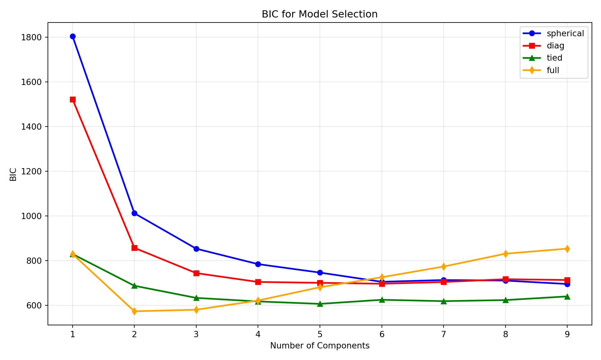
BIC Results:
               spherical         diag        tied        full
Components
1           1804.085438  1522.120153  829.978155  829.978155
2            1012.23518   857.551494   688.09722  574.017833
3            853.823577   744.640361  633.846247  580.861278
4             784.87927   705.134032  618.007065  622.172515
5            747.009336    701.14916  607.156487  681.458987
6            705.808735     697.1752  625.363803  726.149231
7            713.684867   704.851544  619.336283  773.982987
8            711.300242   717.374297  624.071904  831.378879
9            695.945947   713.728296  640.460761   854.01326
# Plot BIC equivalent to plot(mbc, what="BIC")
def plot_bic_selection(bic_matrix, n_components_range, covariance_types):
"""Plot BIC values for model selection"""
plt.figure(figsize=(10, 6))
colors = ['blue', 'red', 'green', 'orange']
markers = ['o', 's', '^', 'd']
for j, (cov_type, color, marker) in enumerate(zip(covariance_types, colors, markers)):
valid_indices = ~np.isnan(bic_matrix[:, j])
if np.any(valid_indices):
plt.plot(np.array(n_components_range)[valid_indices],
bic_matrix[valid_indices, j],
color=color, marker=marker, linewidth=2,
markersize=6, label=f'{cov_type}')
plt.xlabel('Number of Components')
plt.ylabel('BIC')
plt.title('BIC for Model Selection')
plt.legend()
plt.grid(True, alpha=0.3)
plt.tight_layout()
plt.show()
plot_bic_selection(bic_matrix, n_components_range, covariance_types)