5 Types of Statistical Learning
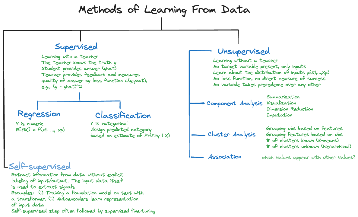
The primary distinction among techniques that learn from data in statistical learning and machine learning is between supervised and unsupervised methods (Figure 5.1). There are other forms of learning:
- With the advent of transformer methods and foundation models, semi-supervised learning has risen in importance.
- Reinforcement learning is used in sequential decision making, for example, when an agent is deciding on a next-best action
5.1 Supervised Learning
Definition: Supervised Learning
Supervised learning trains statistical learning models through a target variable.
Supervised learning is characterized by the presence of a target variable, also called a dependent variable, response variable, or output variable. This is the attribute we wish to model. The training and test data sets contain values for the target variable, in machine learning these values are often called the labels and are described as the “ground truth”. All other variables in the data set are potentially input variables. In short, we know the values of the target variable, now we need to use it in analytical methods to learn how outputs and inputs connect (Figure 5.1).
The goals of supervised learning can be to
- Predict the target variable from input variables.
- Develop a function that approximates the underlying relationship between inputs and outputs.
- Understand the relationship between inputs and outputs.
- Classify observations into categories of the target variable based on the input variables.
- Group the observations into sets of similar data based on the values of the target variable and based on values of the inputs.
- Reduce the dimensionality of the problem by transforming target and inputs from a high-dimensional to a lower-dimensional space.
- Test hypotheses about the target variable.
Studies can pursue one or more of these goals. For example, you might be interested in understanding the relationship between target and input variables and use that relationship for predictions and/or to test hypotheses.
The name supervised learning comes from thinking of learning in an environment that is supervised by a teacher. The teacher asks questions for which they know the correct answer (the ground truth) and judge a student’s response to the questions. The goal is to increase the students knowledge as measured by the quality of their answers. But we do not want students to just memorize answers, we want to teach them to be problem solvers, to apply the knowledge to new problems, to generalize.
The parallel between the description of supervised learning in a classroom and training an algorithm on data is obvious: the problems asked by the teacher, the learning algorithm, are the data points, \(Y\) is the correct answer, the inputs \(x_1,\cdots,x_p\) are the information used by the students to answer the question. The discrepancy between question and answer is measured by \((y - \widehat{y})^2 = (y - \widehat{f}\left( x_1,\cdots x_p \right))^2\) or some other error metric. The training of the model stops when we found a model that generalizes well to previously unseen problems. We are not interested in models that follow the observed data too closely.
Here is a non-exhaustive list of algorithms and models you find in supervised learning.
| Linear regression | Nonlinear regression | Regularized regression (Lasso, Ridge, Elastic nets) |
| Local polynomial regression (LOESS) | Smoothing splines | Kernel methods |
| Logistic regression (binary & binomial) | Multinomial regression (nominal and ordinal) | Poisson regression (counts and rates) |
| Decision trees | Random forests | Bagged trees |
| Adaptive boosting | Gradient boosting machine | Extreme gradient boosting |
| Naïve Bayes classifier | Nearest-neighbor methods | Discriminant analysis (linear and quadratic) |
| Principal component regression | Partial least squares | Generalized linear models |
| Generalized additive models | Mixed models (linear and nonlinear) | Models for correlated data (spatial, time series) |
| Support-vector machines | Neural networks | Extreme gradient boosting |
There is a lot to choose from, and for good reason. The predominant application of data analytics is supervised learning with batch (or mini-batch) data. In batch data analysis the data already exist as a historical data source in one place. We can read all records at once or in segments (called mini-batches). If we have to read the data multiple times, for example, because an iterative algorithm passes through the data at each iteration, we can do so.
Batch-oriented learning contrasts with online learning where the data on which the model is trained is generated and consumed in real time.
5.2 Unsupervised Learning
Definition: Unsupervised Learning
In unsupervised learning methods a target variable is not present.
Unsupervised learning does not utilize a target variable; hence it cannot predict or classify observations. However, we are still interested in discovering structure, patterns, and relationships in the data.
The term unsupervised refers to the fact that we no longer know the ground truth because there is no target variable. Hence the concept of a teacher who knows the correct answers and supervises the learning progress of the student does not apply. In unsupervised learning there are no clear error metrics by which to judge the quality of an analysis, which explains the proliferation of unsupervised methods and the reliance on heuristics. For example, a 5-means cluster analysis will find five groups of observations in the data, whether this is the correct number or not, and it is up to us to interpret what differentiates the groups and to assign group labels. A hierarchical cluster analysis will organize the data hierarchically, whether that makes sense or not.
Often, unsupervised learning is used in an exploratory fashion, improving our understanding of the joint distributional properties of the data and the relationships in the data. The findings then help lead us toward supervised approaches.
A coarse categorization of unsupervised learning techniques also hints at their application:
Association analysis: which values of the variables \(x_{1},\cdots,x_{p}\) tend to occur together in the data? An application is market basket analysis, where the \(X\)s are items are in a shopping cart (or a basket in the market), and \(x_{i} = 1\) if the \(i\)th item is present in the basket and \(x_{i} = 0\) if the item is absent. If items frequently appear together, bread and butter, or beer and chips, for example, then maybe they should be located close together in the store. Association analysis is also useful to build recommender systems: shoppers who bought this item also bought the following items
Cluster analysis: can data be grouped based on \(x_{1},\cdots,x_{p}\) into sets such that the observations within a set are more similar to each other than they are to observations in other sets? Applications of clustering include grouping customers into segments. Segmentation analysis is behind loyalty programs, lower APRs for customers with good credit rating, and churn models.
Dimension reduction: can we transform the inputs \(x_{1},\cdots,x_{p}\) into a set \(c_{1},\cdots,c_{k}\), where \(k \ll p\) without losing relevant information? Applications of dimension reduction are in high-dimensional problems where the number of inputs is large relative to the number of observations. In problems with wide data, the number of inputs \(p\) can be much larger than \(n\), which eliminates many traditional methods of analysis from consideration.
Methods of unsupervised learning often precede supervised learning; the output of an unsupervised learning method can serve as the input to a supervised method. An example is dimension reduction through principal component analysis (PCA, Chapter 24) prior to supervised regression. This technique is known as principal component regression (PCR, Section 8.3.2).
Suppose you have \(n\) observations on a target variable \(Y\) and a large number of potential inputs \(X_1,\cdots,X_p\) where \(p\) is large relative to \(n\). PCA computes linear combinations of the \(p\) inputs that account for decreasing amounts of variability among the \(X\)s. These linear combinations are called the principal components. For example, the first principal component explains 70% of the variability in the inputs, the second principal component explains 20% and the third principal component 5%. Rather than building a regression model with \(p\) predictors, we might use only the first three principal components as inputs in the regression model. The PCA is an unsupervised model because it does not use information about \(Y\) in forming the principal components. The PCR is a supervised method, we want to model the mean of \(Y\) as a function of the \(X\)s. If \(p = 250\), using the first three principal components replaces
\[Y = \beta_{0} + \beta_1 x_1 + \beta_2 x_2 + \beta_3 x_3 + \beta_4 x_4 + \cdots + \beta_{250} x_{250} + \epsilon\]
with
\[Y = \theta_0 + \theta_1 z_1+ \theta_2 z_2 + \theta_3 z_3 + \epsilon\]
where \(z_1\) denotes the first principal component, itself a linear combination of the 250 inputs
\[z_{1} = \phi_1 x_1 + \phi_2 x_2 + \phi_3 x_3 + \cdots + \phi_{250} x_{250}\] \(\text{E}[Y]\) is still a function of all 250 \(X\)s, but indirectly so as the \(Xs\) are represented by linear combinations.