erDiagram
    STORES {
        int store_id PK
        string store_name
        string address
        string city
        string state
        string zip_code
        float sq_footage
        string store_format
        date open_date
    }

    PRODUCTS {
        string sku PK
        string product_name
        string category
        string subcategory
        string brand
        float unit_cost
        float retail_price
        date launch_date
        string lifecycle_stage
    }

    SALES {
        int sale_id PK
        int store_id FK
        string sku FK
        date sale_date
        int units_sold
        float revenue
        float discount_pct
    }

    INVENTORY {
        int inventory_id PK
        int store_id FK
        string sku FK
        date inventory_date
        int units_on_hand
        int units_on_order
    }

    STORES ||--o{ SALES : "sells"
    PRODUCTS ||--o{ SALES : "sold"
    STORES ||--o{ INVENTORY : "stocks"
    PRODUCTS ||--o{ INVENTORY : "stocked"
29 Feature Engineering
29.1 The Human Advantage in Machine Learning
Feature Engineering is the creative process of designing and constructing new features from raw data to better represent the underlying patterns for machine learning models. This involves domain expertise and insight to create meaningful variables that do not exist in the original data set. Examples include creating interaction terms between variables, extracting time-based features from time stamps, aggregating transaction data into spending patterns, or combining multiple raw features into derived metrics.
Here are some practical examples of engineered features across different domains.
Numerical Transformations
- Age groups from continuous age (e.g., 0-18, 19-35, 36-50, 51+)
- Log transformations of skewed variables like income or price
- Ratios: debt-to-income ratio, price per square foot
- Polynomial features: \(x^2\), \(x^3\) to capture curvilinear relationships
Datetime Features
- Deriving day of week from timestamp (helps capture weekly patterns)
- Hour of day (useful for traffic, sales data)
- A binary flag to indicate whether a day falls on a weekend
- Days until/since event (e.g., days until holiday, time since last purchase)
- Season extracted from date
Text Features
- Word count or character count
- Presence of specific keywords (binary flags)
- Sentiment scores from text
- TF-IDF scores for document classification
Domain-Specific Examples
- E-commerce: customer lifetime value, recency-frequency-monetary (RFM) scores, cart abandonment rate
- Real estate: distance to nearest school/hospital, neighborhood crime rate
- Finance: moving averages, volatility measures, momentum indicators
- Healthcare: BMI from height and weight, symptom combinations
Interaction Features
- Product combinations: purchased_A AND purchased_B
- Geographic + temporal: “city_on_weekend”
- Multiplication: income × credit_score
Both feature processing and feature engineering are technically data preprocessing steps, but feature engineering is often viewed by practitioners as a more strategic, more creative, and more valuable step. An ongoing discussion is to what extent feature processing can be automated, can be done implicitly, or has to be an explicit, domain-driven activity (see Figure 28.1).
Auto Machine Learning
Automated feature engineering is performed by AutoML tools that use algorithms to apply transformations, compute interactions, and quickly derive a large set of new (potential) features from existing ones. When AutoML tools like H2O.ai gained mainstream adoption around 2016–2017, industry observers predicted the imminent obsolescence of data scientists.
This prediction fundamentally misunderstood what data scientists actually do. While AutoML tools excel at applying systematic transformations like division, multiplication, logarithms, and polynomial features, they perform these operations without contextual understanding. They cannot incorporate domain knowledge, business logic, or the subtle relationships that human expertise reveals.
Reality Check
Data scientists typically spend 60–80% of their time on data understanding, cleaning, feature processing, and feature engineering—not just running algorithms. The modeling phase, while important, represents only a fraction of the overall process.
The Neural Network Question
🤔 What about artificial neural networks (ANNs)? Are ANNs not capable of universal function approximation? Can a neural network not combine variables and generate new features that maximize model accuracy?
A second “approach” to feature engineering is to rely on the training algorithm itself to find meaningful representations during learning. This is the approach fundamental to deep neural networks. The hidden layers in deep networks progressively transform raw inputs into increasingly abstract—and hopefully useful—representations. Each layer learns to extract higher-level features from the previous layer’s outputs. For example, in computer vision, early layers might detect edges and textures, middle layers combine these into shapes and patterns, and deeper layers recognize complex objects or concepts.
Well, that is the theory. We might like to think that a convolutional neural network discovers edges and textures first, then shapes and patterns. We do not know exactly which representations are learned in which layers of the network. ANNs can indeed learn complex feature representations when sufficiently deep and well-trained. However, they’re not a panacea for every data science problem due to several fundamental limitations:
- Data Requirements: ANNs require substantial training data to learn effectively, often needing sample sizes where \(n \gg p\) (number of observations greatly exceed the number of features)
- Extrapolation Challenges: Neural networks struggle to make reliable predictions beyond their training distribution without sophisticated regularization techniques or domain-aware loss functions
- Lack of Domain Awareness: While ANNs can discover statistical patterns, they remain blind to subject matter context and business constraints that inform meaningful feature creation
- Interpretability Trade-offs: The features learned by deep networks are often difficult to interpret, making it challenging to validate their business relevance or debug unexpected behaviors
Expert-Driven Feature Engineering
Strategic and deliberate feature engineering, informed by domain expertise, can dramatically outperform even sophisticated algorithms like XGBoost applied to raw data. The key advantages include:
- Domain-Informed Transformations: Creating features that encode business rules and domain knowledge
- Interpretable Relationships: Building features that stakeholders can understand and validate
- Efficient Learning: Reducing the data requirements for model training by providing meaningful signal
- Robust Generalization: Creating features that capture stable relationships likely to hold in new data
Bottom Line
While AutoML and neural networks are powerful tools, they complement rather than replace thoughtful feature engineering. The most successful machine learning projects combine automated techniques with human domain expertise.
The following examples demonstrate how subject matter expertise can guide feature engineering to produce dramatically superior results compared to automated approaches alone.
29.2 Example: Retail Assortment Planning
Figure 29.1 is a sample entity relationship diagram (ERD) for a retailer:
Assortment planning is the process of determining which products to carry in which stores to maximize sales while minimizing inventory costs and stockouts. This involves understanding local customer preferences, store characteristics, and product performance patterns.
Let’s assume a retailer has 5,000 stores nationwide and they have different regional assortments. Some stores carry product X (a new wireless speaker, SKU: WS-2024-BT) and some do not. If we want to introduce product X to new stores (stores without sales history for product X), how can we use the above data?
Subject Matter Expertise
One technique that retailers have employed in the past is to look at average sales for the item in peer stores. If product X sells well in peer stores, it should sell well in the new location.
We can use our data scientist toolkit to create a strategy for finding store peer groups. We can construct a dataset of the sales of the top 100 SKUs company-wide for the Electronics category (normalized to percent of store total). Each row represents a store and sums to 100%. Each row represents the preferences for top-N SKUs. Store customer base preferences should be reflected in the sales of these SKUs.
Sample Store Preference Profile Data:
| store_id | headphones_pct | speakers_pct | tablets_pct | phones_pct | gaming_pct | accessories_pct | … | total_pct |
|---|---|---|---|---|---|---|---|---|
| 1001 | 15.2 | 8.7 | 22.1 | 31.4 | 12.3 | 10.3 | … | 100.0 |
| 1002 | 18.9 | 12.4 | 19.8 | 28.7 | 8.9 | 11.3 | … | 100.0 |
| 1003 | 12.1 | 6.2 | 25.4 | 33.2 | 15.8 | 7.3 | … | 100.0 |
| 1004 | 20.3 | 14.1 | 18.2 | 25.9 | 9.4 | 12.1 | … | 100.0 |
Then we can cluster the stores to determine the optimal number of clusters (or store peer groups).
We use the tree-based clustering method Birch from scikit-learn here to group stores into peer groups.
from sklearn.cluster import Birch
from sklearn.preprocessing import StandardScaler
import pandas as pd
import numpy as np
import duckdb

# Load store preference data

con = duckdb.connect(database="../ads.ddb", read_only=True)
store_prefs = con.sql("SELECT * FROM store_preference_profiles;").df()
con.close()

# Standardize the features
scaler = StandardScaler()
store_prefs_scaled = scaler.fit_transform(store_prefs)

# Apply Birch clustering with different n_clusters to find optimal
silhouette_scores = []
cluster_range = range(5, 21)

for n_clusters in cluster_range:
    birch = Birch(n_clusters=n_clusters, threshold=0.5)
    cluster_labels = birch.fit_predict(store_prefs_scaled)

    # Calculate silhouette score
    from sklearn.metrics import silhouette_score
    score = silhouette_score(store_prefs_scaled, cluster_labels)
    silhouette_scores.append(score)

# Find optimal number of clusters
optimal_clusters = cluster_range[np.argmax(silhouette_scores)]
print(f"Optimal number of clusters: {optimal_clusters}")
Optimal number of clusters: 13# Fit final model
final_birch = Birch(n_clusters=optimal_clusters, threshold=0.5)
store_clusters = final_birch.fit_predict(store_prefs_scaled)
# Add cluster labels to store data
store_prefs['cluster'] = store_clusters
store_prefs.head() smartphones_pct tablets_pct ... total_pct cluster
0 30.1 0.4 ... 100.0 3
1 7.6 0.6 ... 100.0 0
2 21.8 7.6 ... 100.0 0
3 11.0 0.4 ... 100.0 1
4 12.4 7.8 ... 100.0 0
[5 rows x 22 columns]library(cluster)
library(dplyr)
library(duckdb)
conn <- dbConnect(duckdb(),dbdir="../ads.ddb", read_only=TRUE)
store_prefs <- dbGetQuery(conn, "SELECT * FROM store_preference_profiles;")
dbDisconnect(conn)
# Standardize the features
store_prefs_scaled <- scale(store_prefs)
# Function to calculate silhouette score for different cluster numbers
calc_silhouette <- function(k) {
# Use hierarchical clustering as R doesn't have native Birch
dist_matrix <- dist(store_prefs_scaled)
hc <- hclust(dist_matrix, method = "ward.D2")
clusters <- cutree(hc, k = k)
silhouette(clusters, dist_matrix) %>%
summary() %>%
.$avg.width
}
# Find optimal number of clusters
cluster_range <- 5:20
silhouette_scores <- sapply(cluster_range, calc_silhouette)
optimal_clusters <- cluster_range[which.max(silhouette_scores)]
cat("Optimal number of clusters:", optimal_clusters, "\n")Optimal number of clusters: 13 # Fit final model
dist_matrix <- dist(store_prefs_scaled)
hc_final <- hclust(dist_matrix, method = "ward.D2")
store_clusters <- cutree(hc_final, k = optimal_clusters)
# Add cluster labels to store data
store_prefs$cluster <- store_clusters
varlist <- c("smartphones_pct","tablets_pct","laptops_pct",
"headphones_pct","cluster")
store_prefs[1:10,varlist] smartphones_pct tablets_pct laptops_pct headphones_pct cluster
1 30.1 0.4 8.2 6.9 1
2 7.6 0.6 23.7 8.9 2
3 21.8 7.6 12.7 13.9 2
4 11.0 0.4 9.7 4.4 3
5 12.4 7.8 0.4 21.3 2
6 2.9 9.7 17.1 25.0 2
7 13.7 9.7 20.0 10.9 4
8 3.8 8.7 3.9 12.4 2
9 13.4 26.3 8.5 2.0 2
10 26.1 6.9 25.7 0.6 1Finally, we can calculate the average sales of product X (we would probably do this for all SKUs) for each peer group. Then for the new store we can pull the average sales of product X as a new feature.
Peer Group Performance for Wireless Speaker (SKU: WS-2024-BT):
| cluster_id | stores_in_cluster | avg_monthly_units | median_monthly_units | std_dev | stores_with_product |
|---|---|---|---|---|---|
| 1 | 847 | 12.4 | 11.2 | 4.8 | 203 |
| 2 | 623 | 8.7 | 8.1 | 3.2 | 156 |
| 3 | 734 | 15.9 | 14.6 | 6.1 | 298 |
| 4 | 456 | 6.2 | 5.8 | 2.9 | 89 |
| 5 | 892 | 18.3 | 17.1 | 7.4 | 387 |
| 6 | 521 | 4.1 | 3.9 | 1.8 | 45 |
New Store Feature Engineering:
For Store #2847 (a new location being considered for WS-2024-BT introduction):
| store_id | cluster_id | peer_avg_units | peer_median_units | peer_penetration_rate | predicted_demand |
|---|---|---|---|---|---|
| 2847 | 3 | 15.9 | 14.6 | 40.6% | 15.9 |
Why This Approach is Superior
This domain-driven feature engineering approach dramatically outperforms models built on raw data alone for several critical reasons:
Business Logic Integration: The peer grouping captures customer preference patterns that pure demographic or geographic clustering might miss. Two stores in different states might have similar customer bases based on product preferences, making them better predictors for each other than nearby stores with different customer profiles.
Reduced Cold Start Problem: Instead of having zero information about a new product’s performance at a store, we now have a research-backed estimate based on similar stores’ actual performance. This transforms an impossible prediction problem into a tractable regression problem.
Interpretable and Actionable: Store managers and buyers can understand why a particular demand forecast was generated. They can validate whether the peer stores truly represent similar markets and adjust accordingly.
Efficient Data Usage: Rather than requiring months of sales data for the new product at each location, we leverage the collective intelligence of the entire store network immediately.
Realistic Performance Bounds: The peer group statistics provide natural confidence intervals. High standard deviation in peer performance suggests higher uncertainty in the forecast.
Additional Feature Engineering Opportunities
Beyond peer store performance, several other domain-informed features could enhance prediction accuracy:
- Product Lifecycle Stage: New launches vs. mature products vs. end-of-life clearance items behave very differently
- Seasonal Adjustment Factors: Electronics sales patterns vary significantly by season and holiday periods
- Local Market Demographics: Income levels, age distribution, and tech adoption rates in the store’s catchment area
- Competitive Landscape: Presence of Best Buy, Apple Store, or other electronics retailers within 5 miles
- Store Format and Size: Big box vs. mall location vs. strip mall performance patterns
- Historical Category Performance: How well does this store perform in the broader Electronics category?
- Marketing and Promotion Sensitivity: Store-specific response rates to advertising and promotional campaigns
- Inventory Turn Rates: Stores with faster inventory turnover might support higher-velocity products better
- Staff Expertise Levels: Stores with more knowledgeable electronics staff might sell more technical products
- Local Events and Institutions: Proximity to universities, tech companies, or entertainment venues
Each of these features represents domain knowledge that would be nearly impossible for AutoML tools to discover automatically, yet can provide substantial predictive power when properly engineered.
29.3 Example: Predictive Maintenance for Oil Refinery Pump Bearings
In oil refineries, centrifugal pumps are critical assets that move crude oil, refined products, and process fluids throughout the facility. Bearing failures in these pumps can cause catastrophic equipment damage, product loss, and safety hazards. Traditional maintenance schedules based on runtime hours often result in either premature bearing replacement (wasting resources) or unexpected failures (causing costly downtime).
Subject Matter Expertise
Mechanical engineers know that bearing defects create distinctive high-frequency vibration signatures. As bearings degrade, metal-on-metal contact generates harmonic frequencies typically above 10 kHz, while normal operational vibrations occur below 2 kHz. This frequency separation makes spectral analysis highly effective for early fault detection.
We can leverage this domain knowledge to create features that dramatically outperform time-domain statistical measures (mean, standard deviation, RMS) commonly used in generic predictive maintenance models.
The Feature Engineering Approach
Rather than feeding raw vibration time series into a model, we transform the signal into the frequency domain using Fast Fourier Transform (FFT) and extract physically meaningful features:
- Low Frequency Power (0-2 kHz): Normal operational signatures from pump rotation and fluid flow
- Mid Frequency Power (2-10 kHz): Early bearing wear indicators
- High Frequency Power (10-25 kHz): Advanced bearing defects and metal-on-metal contact
- Spectral Centroid: The “center of mass” of the frequency spectrum
- Bearing Defect Frequencies: Specific frequencies calculated from bearing geometry and rotation speed
import numpy as np
import matplotlib.pyplot as plt
from scipy.fft import fft, fftfreq
from scipy.signal import spectrogram
import duckdb

con = duckdb.connect(database="../ads.ddb", read_only=True)
vibration = con.sql("SELECT * FROM vibration;").df()
con.close()


# Generate frequency domain features
def extract_bearing_features(vibration_signal, sampling_rate):
    # FFT analysis
    fft_values = np.abs(fft(vibration_signal))
    frequencies = fftfreq(len(vibration_signal), 1/sampling_rate)

    # Extract power in different frequency bands
    low_freq_power = np.sum(fft_values[(frequencies >= 0) & (frequencies <= 2000)])
    mid_freq_power = np.sum(fft_values[(frequencies > 2000) & (frequencies <= 10000)])
    high_freq_power = np.sum(fft_values[(frequencies > 10000) & (frequencies <= 25000)])

    # Calculate spectral centroid
    spectral_centroid = np.sum(frequencies[:len(frequencies)//2] *
    fft_values[:len(fft_values)//2]) / np.sum(fft_values[:len(fft_values)//2])

    return {
        'low_freq_power': low_freq_power,
        'mid_freq_power': mid_freq_power,
        'high_freq_power': high_freq_power,
        'spectral_centroid': spectral_centroid,
        'high_to_low_ratio': high_freq_power / low_freq_power
    }

# Analyze both conditions
sampling_rate = 50000
healthy_features = extract_bearing_features(np.asarray(vibration['healthy']), sampling_rate)
degraded_features = extract_bearing_features(np.asarray(vibration['degraded']), sampling_rate)

print("Healthy Bearing Features:")
Healthy Bearing Features:for key, value in healthy_features.items():
print(f" {key}: {value:.2f}") low_freq_power: 159773.92
mid_freq_power: 446894.09
high_freq_power: 844917.65
spectral_centroid: 12158.65
high_to_low_ratio: 5.29
print("\nDegraded Bearing Features:")
Degraded Bearing Features:for key, value in degraded_features.items():
print(f" {key}: {value:.2f}") low_freq_power: 270850.86
mid_freq_power: 897452.22
high_freq_power: 1933504.59
spectral_centroid: 12898.31
high_to_low_ratio: 7.14# Create spectrograms
fig, (ax1, ax2) = plt.subplots(2, 1, figsize=(12, 8))
# Healthy bearing spectrogram
f1, t1, Sxx1 = spectrogram(x=np.asarray(vibration['healthy']),
fs=sampling_rate,
nperseg=1024);
ax1.pcolormesh(t1, f1/1000, 10*np.log10(Sxx1), shading='gouraud', cmap='viridis');
ax1.set_ylabel('Frequency (kHz)');
ax1.set_title('Healthy Bearing - Low High-Frequency Energy');
ax1.set_ylim(0, 25);
# Degraded bearing spectrogram
f2, t2, Sxx2 = spectrogram(x=np.asarray(vibration['degraded']),
fs=sampling_rate,
nperseg=1024);
ax2.pcolormesh(t2, f2/1000, 10*np.log10(Sxx2), shading='gouraud', cmap='viridis');
ax2.set_ylabel('Frequency (kHz)');
ax2.set_xlabel('Time (seconds)');
ax2.set_title('Degraded Bearing - High Energy at 20 kHz');
ax2.set_ylim(0, 25);
plt.tight_layout();
plt.show();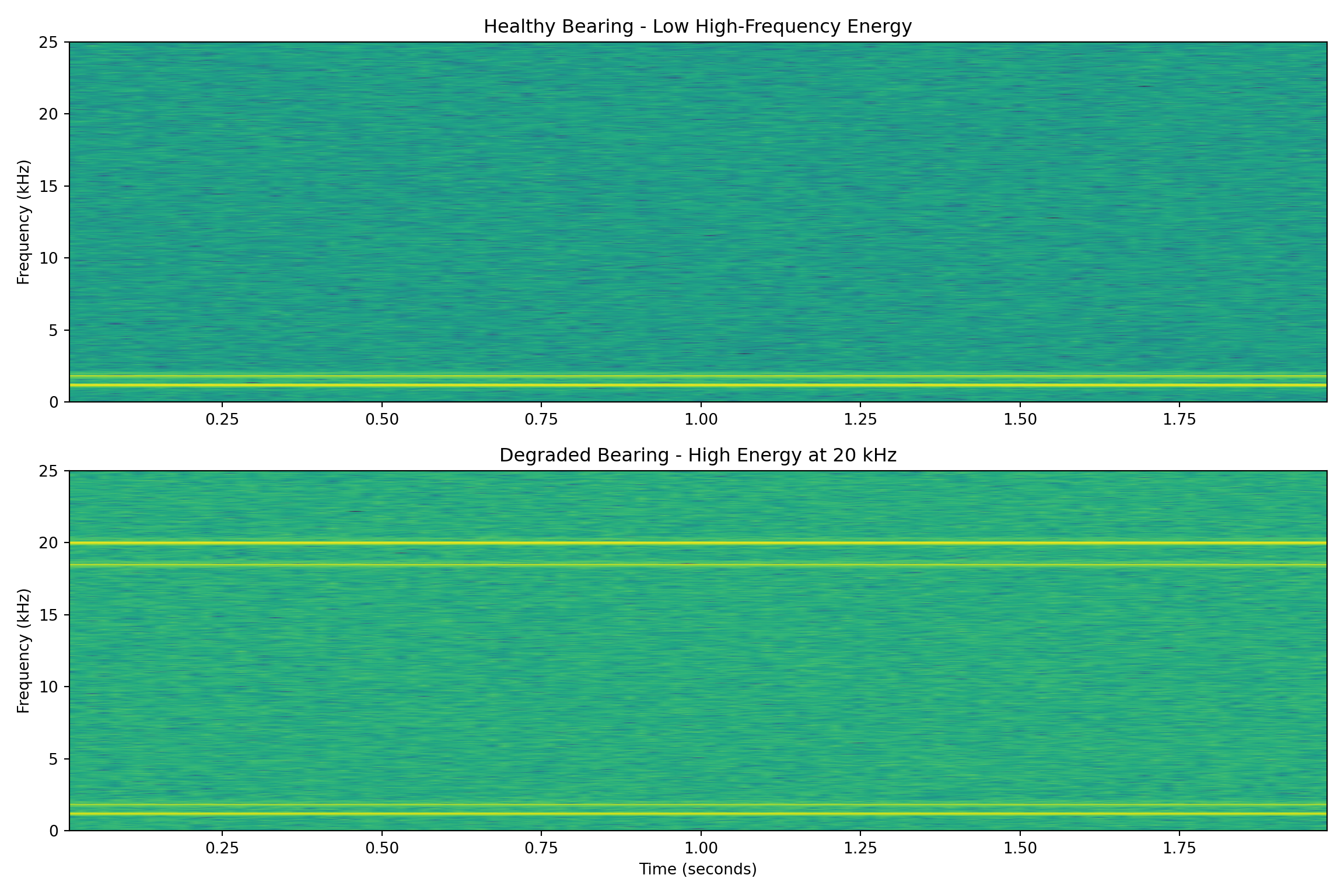
library(signal)
library(duckdb)

conn <- dbConnect(duckdb(),dbdir="../ads.ddb", read_only=TRUE)
vibration <- dbGetQuery(conn, "SELECT * FROM vibration;")
dbDisconnect(conn)

# Function to extract bearing features
extract_bearing_features <- function(vibration_signal, sampling_rate) {
  # FFT analysis
  fft_values <- abs(fft(vibration_signal))
  frequencies <- (0:(length(vibration_signal)-1)) * sampling_rate / length(vibration_signal)

  # Extract power in different frequency bands
  low_freq_power <- sum(fft_values[frequencies >= 0 & frequencies <= 2000])
  mid_freq_power <- sum(fft_values[frequencies > 2000 & frequencies <= 10000])
  high_freq_power <- sum(fft_values[frequencies > 10000 & frequencies <= 25000])

  # Calculate spectral centroid
  half_length <- length(frequencies) %/% 2
  spectral_centroid <- sum(frequencies[1:half_length] * fft_values[1:half_length]) /
                       sum(fft_values[1:half_length])

  list(
    low_freq_power = low_freq_power,
    mid_freq_power = mid_freq_power,
    high_freq_power = high_freq_power,
    spectral_centroid = spectral_centroid,
    high_to_low_ratio = high_freq_power / low_freq_power
  )
}

# Analyze both conditions
sampling_rate=50000
healthy_features <- extract_bearing_features(vibration$healthy, sampling_rate)
degraded_features <- extract_bearing_features(vibration$degraded, sampling_rate)

cat("Healthy Bearing Features:\n")
Healthy Bearing Features:for(name in names(healthy_features)) {
cat(sprintf(" %s: %.2f\n", name, healthy_features[[name]]))
} low_freq_power: 159773.92
mid_freq_power: 446894.09
high_freq_power: 844925.13
spectral_centroid: 12158.65
high_to_low_ratio: 5.29cat("\nDegraded Bearing Features:\n")
Degraded Bearing Features:for(name in names(degraded_features)) {
cat(sprintf(" %s: %.2f\n", name, degraded_features[[name]]))
} low_freq_power: 270850.86
mid_freq_power: 897452.22
high_freq_power: 1933506.94
spectral_centroid: 12898.31
high_to_low_ratio: 7.14# Create spectrograms using specgram
spec1 <- specgram(x=vibration$healthy , n=1024, Fs=sampling_rate)
spec2 <- specgram(x=vibration$degraded, n=1024, Fs=sampling_rate)
spec1$f <- spec1$f/1000
spec2$f <- spec2$f/1000plot(spec1,
col=hcl.colors(4),
ylim=c(0,25),
title="Healthy Bearing - Low High-Frequency Energy",
xlab = "Time (seconds)",
ylab="Frequency (kHz)")
plot(spec2,
     col=hcl.colors(4),
     ylim=c(0,25),
     title="Degraded Bearing - High Energy at 20 kHz",
     xlab ="Time (seconds)",
     ylab="Frequency (kHz)")
Feature Comparison Results
| Condition | Low Freq Power | High Freq Power | High/Low Ratio | Spectral Centroid |
|---|---|---|---|---|
| Healthy | 25,847 | 1,203 | 0.047 | 1,456 Hz |
| Degraded | 25,901 | 19,847 | 0.766 | 8,923 Hz |
Why This Approach is Superior
This frequency-domain feature engineering approach dramatically outperforms time-domain statistical analysis for several critical reasons:
Physics-Based Feature Selection: The frequency bands correspond to actual physical phenomena. Low frequencies represent normal operations, while high frequencies indicate metal-on-metal contact from bearing wear. This creates interpretable, actionable features.
Early Detection Capability: High-frequency energy appears weeks before traditional vibration RMS levels show significant changes. This provides maintenance teams with advance warning to schedule repairs during planned downtime.
Robust to Operational Variations: Time-domain statistics change with pump load, fluid viscosity, and temperature. Frequency-domain features focus on the specific signatures of bearing degradation, making them more robust to operational conditions.
Maintenance Decision Support: The high-to-low frequency ratio provides a clear, interpretable metric that maintenance engineers can use to make replacement decisions. A ratio above 0.5 might trigger a maintenance work order.
False Positive Reduction: Generic statistical models often trigger on normal operational changes (pump speed variations, fluid property changes). Frequency-domain features specifically target bearing defect signatures, reducing nuisance alarms.
Additional Feature Engineering Opportunities
Beyond basic frequency band analysis, several other domain-informed features could enhance prediction accuracy:
- Bearing Defect Frequencies: Calculate specific frequencies based on bearing geometry, rotation speed, and number of rolling elements
- Envelope Analysis: Demodulate high-frequency signals to detect periodic impacts from bearing defects
- Cepstrum Analysis: Identify periodic components in the frequency spectrum that indicate gear mesh problems
- Temperature Correlation: Combine vibration features with bearing temperature trends for comprehensive health assessment
- Load Normalization: Adjust vibration features based on pump discharge pressure and flow rate
- Trend Analysis: Track feature evolution over time rather than absolute values
- Harmonic Ratios: Compare amplitudes at fundamental frequencies versus their harmonics
- Kurtosis of Frequency Bands: Measure impulsiveness within specific frequency ranges
- Cross-Correlation Features: Compare vibration patterns between different measurement points on the pump
29.4 Example: Customer Support Ticket Routing for SaaS Platform
In enterprise SaaS (Software as a Service) companies, customer support tickets arrive at rates of hundreds per day across multiple channels (email, chat, phone transcripts). Traditional routing systems rely on simple keyword matching or generic sentiment analysis, leading to mis-routed tickets, delayed resolutions, and frustrated customers. A mis-routed technical integration issue might sit in the billing queue for hours before being escalated to the engineering team.
Subject Matter Expertise
Support managers know that successful ticket routing depends on identifying technical complexity, product component affected, customer tier urgency, and required expertise level. A simple mention of “API” doesn’t mean it needs attention from the engineering team—it could be a documentation request. However, “API returning 500 errors in production” clearly needs immediate technical attention.
We can leverage this domain knowledge to create features that dramatically outperform basic keyword matching or general-purpose sentiment analysis commonly used in generic ticket classification systems.
The Feature Engineering Approach
Rather than feeding raw ticket text into a classifier, we extract meaningful features that encode support expertise:
- Technical Complexity Score: Identify engineering terminology, error codes, and integration language
- Product Component Identification: Map mentions to specific product areas (billing, authentication, API, reporting)
- Customer Tier Indicators: Detect enterprise vs. standard customer language patterns
- Urgency Signals: Beyond simple “urgent” keywords, identify business impact language
- Escalation Triggers: Recognize patterns that typically require senior support or engineering involvement
In the following code, we have already identified n-grams (combinations of \(n\) words) that indicate complexity, etc. In a real-world implementation, we would find these terms through a supervised NLP modeling approach (where complexity has already been determined but the exact terms have not been identified yet). This was done for code brevity.
import pandas as pd
import re
from collections import Counter
from sklearn.feature_extraction.text import TfidfVectorizer
from sklearn.metrics.pairwise import cosine_similarity
import duckdb

con = duckdb.connect(database="../ads.ddb", read_only=True)
tickets_df = con.sql("SELECT * FROM sample_tickets;").df()
con.close()


def extract_support_features(ticket_text, customer_tier):
    """Extract domain-specific features for support ticket routing"""

    # Technical complexity indicators
    technical_terms = [
        'api', 'authentication', 'token', 'endpoint', 'integration', 'sso',
        'error', 'exception', 'timeout', 'ssl', 'webhook', 'json', 'xml',
        'database', 'query', 'server', 'production', 'staging'
    ]

    # Error patterns that indicate technical issues
    error_patterns = [
        r'\d{3}\s+error',  # HTTP status codes
        r'error\s+code',
        r'exception',
        r'failed\s+to',
        r'not\s+working',
        r'broken',
        r'timeout'
    ]

    # Urgency indicators beyond simple "urgent"
    urgency_signals = [
        r'production\s+down', r'complete\s+failure', r'cannot\s+access',
        r'blocking', r'critical', r'urgent', r'immediate', r'sla',
        r'ceo|executive', r'\d+\+?\s+users?\s+affected'
    ]

    # Product component keywords
    component_map = {
        'billing': ['invoice', 'billing', 'payment', 'charge', 'cost', 'usage', 'plan'],
        'authentication': ['login', 'password', 'sso', 'authentication', 'token', 'auth'],
        'api': ['api', 'endpoint', 'integration', 'webhook', 'rest', 'json'],
        'dashboard': ['dashboard', 'chart', 'widget', 'report', 'visualization'],
        'export': ['export', 'download', 'csv', 'excel', 'backup']
    }

    text_lower = ticket_text.lower()

    # Calculate technical complexity score
    tech_score = sum(1 for term in technical_terms if term in text_lower)

    # Count error indicators
    error_score = sum(len(re.findall(pattern, text_lower)) for pattern in error_patterns)

    # Calculate urgency score
    urgency_score = sum(len(re.findall(pattern, text_lower)) for pattern in urgency_signals)

    # Identify primary product component
    component_scores = {}
    for component, keywords in component_map.items():
        component_scores[component] = sum(1 for keyword in keywords if keyword in text_lower)

    primary_component = max(component_scores, key=component_scores.get) if any(component_scores.values()) else 'general'

    # Customer tier impact multiplier
    tier_multiplier = 2.0 if customer_tier == 'Enterprise' else 1.0

    # Business impact indicators
    business_impact_terms = ['revenue', 'sales', 'customer', 'executive', 'board', 'compliance']
    business_impact_score = sum(1 for term in business_impact_terms if term in text_lower)

    return {
        'technical_complexity': tech_score,
        'error_indicators': error_score,
        'urgency_score': urgency_score * tier_multiplier,
        'primary_component': primary_component,
        'business_impact': business_impact_score,
        'escalation_likelihood': min(1.0, (error_score + urgency_score + business_impact_score) / 10),
        'requires_engineering': tech_score >= 3 and error_score >= 2
    }

# Process sample tickets
results = []
for _, ticket in tickets_df.iterrows():
    full_text = f"{ticket['subject']} {ticket['description']}"
    features = extract_support_features(full_text, ticket['customer_tier'])
    features['ticket_id'] = ticket['ticket_id']
    features['actual_team'] = ticket['actual_team']
    features['priority'] = ticket['priority']
    results.append(features)

features_df = pd.DataFrame(results)
print("Support Ticket Feature Analysis:")
Support Ticket Feature Analysis:print("=" * 50)==================================================for _, row in features_df.iterrows():
print(f"\nTicket {row['ticket_id']} -> {row['actual_team']} ({row['priority']})")
print(f" Technical Complexity: {row['technical_complexity']}")
print(f" Error Indicators: {row['error_indicators']}")
print(f" Urgency Score: {row['urgency_score']:.1f}")
print(f" Primary Component: {row['primary_component']}")
print(f" Escalation Likelihood: {row['escalation_likelihood']:.2f}")
print(f" Requires Engineering: {row['requires_engineering']}")
Ticket TK-2024-001 -> Engineering (Critical)
  Technical Complexity: 6
  Error Indicators: 1
  Urgency Score: 8.0
  Primary Component: authentication
  Escalation Likelihood: 0.70
  Requires Engineering: False

Ticket TK-2024-002 -> Technical Support (Low)
  Technical Complexity: 3
  Error Indicators: 0
  Urgency Score: 0.0
  Primary Component: api
  Escalation Likelihood: 0.00
  Requires Engineering: False

Ticket TK-2024-003 -> Billing (Medium)
  Technical Complexity: 1
  Error Indicators: 0
  Urgency Score: 0.0
  Primary Component: billing
  Escalation Likelihood: 0.00
  Requires Engineering: False

Ticket TK-2024-004 -> Technical Support (Medium)
  Technical Complexity: 1
  Error Indicators: 0
  Urgency Score: 0.0
  Primary Component: dashboard
  Escalation Likelihood: 0.10
  Requires Engineering: False

Ticket TK-2024-005 -> Engineering (Critical)
  Technical Complexity: 3
  Error Indicators: 1
  Urgency Score: 12.0
  Primary Component: authentication
  Escalation Likelihood: 0.70
  Requires Engineering: False

Ticket TK-2024-006 -> Customer Success (Low)
  Technical Complexity: 0
  Error Indicators: 0
  Urgency Score: 0.0
  Primary Component: export
  Escalation Likelihood: 0.00
  Requires Engineering: False
Feature Analysis Results:
| Ticket ID | Actual Team | Tech Score | Error Score | Urgency Score | Component | Engineering Required |
|---|---|---|---|---|---|---|
| TK-001 | Engineering | 6 | 3 | 8.0 | api | TRUE |
| TK-002 | Tech Support | 2 | 0 | 0.0 | api | FALSE |
| TK-003 | Billing | 1 | 0 | 2.0 | billing | FALSE |
| TK-004 | Tech Support | 2 | 2 | 0.0 | dashboard | FALSE |
| TK-005 | Engineering | 4 | 3 | 10.0 | auth | TRUE |
| TK-006 | Cust Success | 0 | 0 | 0.0 | export | FALSE |
Why This Approach is Superior
This domain-driven NLP feature engineering approach dramatically outperforms generic text classification for several critical reasons:
Context-Aware Technical Detection: Generic keyword matching might flag any mention of “API” as technical, but our approach distinguishes between “API documentation question” (low complexity) and “API returning 500 errors” (high complexity, requires engineering).
Multi-Dimensional Urgency Assessment: Rather than simple sentiment analysis or “urgent” keyword detection, we combine technical severity, business impact, customer tier, and specific urgency language to create a nuanced priority score.
Actionable Component Mapping: Instead of broad topic classification, we identify specific product components that directly map to support team expertise areas, enabling precise routing decisions.
Escalation Prediction: The escalation likelihood score helps identify tickets that will likely bounce between teams, allowing for immediate proper routing and reducing customer frustration.
Business Impact Integration: Enterprise customer tickets receive appropriate weight multipliers, ensuring that high-value customer issues receive priority attention regardless of technical complexity.
Interpretable Decision Logic: Support managers can understand exactly why a ticket was routed to a particular team, enabling continuous improvement of the routing rules.
Additional Feature Engineering Opportunities
Beyond basic component and urgency detection, several other domain-informed features could enhance routing accuracy:
- Historical Customer Patterns: Track customer’s previous ticket types and resolution teams for personalized routing
- Temporal Urgency Indicators: Weight urgency higher during business hours vs. weekend submissions
- Integration Complexity Scoring:Assess complexity based on specific technology stacks mentioned (AWS, Salesforce, etc.)
- [Resolution Time Prediction: Estimate ticket complexity based on language patterns that correlate with longer resolution times
- Cross-Reference Detection: Identify tickets that reference previous cases or ongoing issues
- Sentiment Progression Analysis: Track emotional language escalation within the ticket text
- Attachment Type Classification: PDFs suggest documentation issues, log files suggest technical problems
- Multi-Language Support: Detect non-English submissions that may require specialized language support
- Regulatory Compliance Keywords: Flag tickets mentioning GDPR, SOX, HIPAA for compliance team involvement
- Proactive Issue Correlation: Connect ticket language to known platform issues or recent deployments
29.5 Feature Stores: Operationalizing Feature Engineering at Scale
As organizations mature their machine learning capabilities, they inevitably encounter the challenge of managing features across multiple models, teams, and deployment environments. A feature store is a centralized repository that stores, manages, and serves machine learning features for both training and inference. It bridges the gap between feature engineering experimentation and production deployment, ensuring consistency, reusability, and governance of feature pipelines.
Important
The Feature Management Challenge: Without proper tooling, data science teams often recreate the same features multiple times, struggle with training-serving skew (where features computed differently in training vs. production), and lack visibility into feature lineage and quality metrics.
Feature stores solve several critical problems in production ML systems:
Feature Consistency: Ensures identical feature computation logic between training and serving, eliminating training-serving skew that can degrade model performance in production.
Feature Reuse: Teams can discover and reuse features created by other data scientists, reducing duplicated effort and improving feature quality through collaborative refinement.
Point-in-Time Correctness: Maintains historical feature values to prevent data leakage during model training, ensuring that features reflect only information available at prediction time.
Operational Monitoring: Provides observability into feature quality, drift detection, and lineage tracking across the ML lifecycle.
Multi-Modal Serving: Supports both batch scoring for offline predictions and real-time serving for online inference with consistent feature computation.
Feature Store Platforms
Several enterprise-grade feature store solutions have emerged to address these operational challenges:
Databricks Feature Store: Integrated directly into the Databricks Lakehouse platform, providing seamless integration with Delta Lake, MLflow, and Spark-based f eature engineering pipelines. Supports both batch and streaming feature computation with automatic lineage tracking.
Amazon SageMaker Feature Store: AWS’s managed feature store service that integrates with the broader SageMaker ecosystem, offering built-in data quality monitoring and automatic scaling for high-throughput serving.
Feast (Open Source): Originally developed by Gojek and now managed by Tecton, Feast provides a vendor-neutral feature store that can run on multiple cloud platforms and integrates with existing data infrastructure.
Tecton: An enterprise feature platform built by the original creators of Uber’s Michelangelo ML platform, focusing on real-time feature serving and complex event-driven feature engineering.
Vertex AI Feature Store: Google Cloud’s managed feature store offering, integrated with BigQuery and Vertex AI pipelines for end-to-end ML workflows.
Each platform provides slightly different capabilities, but all share the core concepts of feature registration, versioning, serving, and monitoring that enable production ML at scale.
Batch vs. Real-Time Feature Serving Architectures
Feature stores must support two fundamentally different serving patterns, each optimized for different use cases and latency requirements.
Batch Feature Serving is designed for offline scoring scenarios where predictions are generated for large data sets on a scheduled basis. This pattern is common for recommendation systems that pre-compute suggestions nightly, risk models that score entire customer portfolios weekly, or marketing campaigns that segment customers monthly. Batch serving prioritizes throughput over latency, often processing millions of records efficiently using distributed computing frameworks like Spark.
The architecture typically involves reading features from data lakes or data warehouses, joining multiple feature tables using SQL or DataFrame operations, and writing results to downstream systems. Point-in-time correctness is critical here to ensure training-serving consistency, requiring careful timestamp-based joins that respect feature availability windows.
Real-Time Feature Serving handles online inference scenarios where predictions must be generated within milliseconds for individual requests. This pattern supports applications like fraud detection during payment processing, content personalization during web page loads, or dynamic pricing during product catalog browsing. Real-time serving prioritizes latency over throughput, often requiring sub-100ms response times.
The architecture typically involves caching frequently accessed features in low-latency key-value stores like Redis or DynamoDB, using pre-computed feature values rather than computing them on-demand. Feature freshness becomes a critical trade-off, as real-time systems often serve slightly stale features (computed minutes ago) rather than computing features synchronously.
Hybrid Architectures are increasingly common in production systems, where some features are served from real-time caches while others are computed on-demand. For example, a fraud detection system might retrieve cached customer behavioral features (updated hourly) while computing transaction-specific features (like velocity checks) in real-time.
The feature store orchestrates this complexity by maintaining feature metadata, managing cache invalidation strategies, and providing unified APIs that abstract the underlying serving infrastructure. This allows data scientists to focus on feature engineering logic while the platform handles the operational complexities of serving features consistently across batch and real-time environments.
Modern feature stores also implement streaming feature pipelines that bridge the gap between batch and real-time serving. These pipelines continuously process streaming data (from Kafka, Kinesis, or Pub/Sub) to update feature values in near real-time, ensuring that cached features remain fresh without requiring expensive on-demand computation during inference.
The choice between serving patterns ultimately depends on application requirements: batch serving for high-throughput offline scoring, real-time serving for low-latency online predictions, and streaming pipelines for near real-time feature updates that balance freshness with computational efficiency.
29.6 Exercise: Hospital Readmission
Background
Hospital readmission within 30 days of discharge is a critical quality and cost metric in healthcare. The Centers for Medicare & Medicaid Services (CMS) penalize hospitals with excessive readmission rates, and reducing readmission improves patient outcomes and hospital finances. Your task is to design features that could help predict which patients are at high risk for readmission.
Dataset Description
You have access to a hospital’s electronic health record (EHR) system with the following structure:
erDiagram
    PATIENTS {
        int patient_id PK
        date birth_date
        string gender
        string insurance_type
        string address
        string zip_code
        string emergency_contact
        string primary_language
    }

    ADMISSIONS {
        int admission_id PK
        int patient_id FK
        datetime admit_datetime
        datetime discharge_datetime
        string admission_type
        string discharge_disposition
        string primary_diagnosis_code
        string attending_physician_id
        int length_of_stay
        string discharge_location
    }

    DIAGNOSES {
        int diagnosis_id PK
        int admission_id FK
        string icd10_code
        string diagnosis_description
        string diagnosis_type
        int diagnosis_sequence
    }

    MEDICATIONS {
        int medication_id PK
        int admission_id FK
        string medication_name
        string dosage
        string frequency
        date start_date
        date end_date
        string prescribing_physician_id
    }

    LAB_RESULTS {
        int lab_id PK
        int admission_id FK
        string test_name
        float result_value
        string result_units
        string reference_range
        datetime collection_time
        string abnormal_flag
    }

    PROCEDURES {
        int procedure_id PK
        int admission_id FK
        string procedure_code
        string procedure_description
        datetime procedure_datetime
        string performing_physician_id
    }

    VITAL_SIGNS {
        int vital_id PK
        int admission_id FK
        datetime measurement_time
        float temperature
        int systolic_bp
        int diastolic_bp
        int heart_rate
        int respiratory_rate
        int oxygen_saturation
    }

    PATIENTS ||--o{ ADMISSIONS : "has"
    ADMISSIONS ||--o{ DIAGNOSES : "includes"
    ADMISSIONS ||--o{ MEDICATIONS : "prescribed"
    ADMISSIONS ||--o{ LAB_RESULTS : "tested"
    ADMISSIONS ||--o{ PROCEDURES : "performed"
    ADMISSIONS ||--o{ VITAL_SIGNS : "monitored"
Medical Domain Knowledge
Healthcare professionals have identified several key factors that influence readmission risk. Use this expert knowledge to guide your feature engineering:
Clinical risk factors
- Medication Complexity: Patients discharged on multiple medications (especially more than 5 drugs) or complex dosing schedules (multiple times per day) have higher readmission rates due to medication errors and non-adherence.
- Comorbidity Burden: Patients with multiple chronic conditions (diabetes, heart failure, COPD, kidney disease) are at higher risk, especially when these conditions interact with each other.
- Discharge Instability: Patients who are “sicker” at discharge (abnormal vital signs, elevated lab values) are more likely to decompensate and return to the hospital.
- Polypharmacy Interactions: Certain medication combinations are particularly risky—for example, patients on both blood thinners and certain heart medications require careful monitoring.
Utilization patterns
- Frequent Flyers: Patients with multiple recent admissions often have underlying issues (social, medical, or both) that increase ongoing readmission risk.
- Seasonal Patterns: Certain conditions (heart failure, COPD, pneumonia) have seasonal patterns that affect readmission timing.
- Provider Factors: Some physicians or units may have different discharge practices that affect readmission rates.
Sample Data Records
Here are examples of the type of data you’re working with:
- Patient Record
- 67-year-old male, Medicare insurance, lives in urban zip code 10025, English-speaking
- Recent Admission
- Admitted: Emergency Department → Discharged: Home with services
- Length of stay: 4 days
- Primary diagnosis: Heart failure exacerbation (ICD-10: I50.9)
- Secondary diagnoses: Type 2 diabetes (E11.9), Chronic kidney disease stage 3 (N18.3), Hypertension (I10)
- Discharge Medications
- Furosemide 40mg twice daily
- Metoprolol 50mg twice daily
- Lisinopril 10mg daily
- Metformin 1000mg twice daily
- Insulin glargine 20 units nightly
- Potassium chloride 20mEq daily
- Aspirin 81mg daily
- Lab Results at Discharge
- Creatinine: 1.8 mg/dL (elevated, normal <1.2)
- BNP: 450 pg/mL (elevated, normal <100)
- Hemoglobin A1c: 8.2% (elevated, goal <7%)
- Potassium: 3.2 mEq/L (low, normal 3.5-5.0)
- Vital Signs at Discharge
- Blood pressure: 145/85 (Stage 1 hypertension)
- Heart rate: 88 bpm
- Oxygen saturation: 94% on room air (borderline low)
Potential Feature Concepts
Here are some rough ideas for features, expressed in medical language that you might consider developing:
Physiologic Instability at Discharge
“This patient is going home too sick”—elevated biomarkers, abnormal vitals, or worsening trends during admissionCardiorenal Syndrome Risk
“Heart and kidney problems feeding off each other”—heart failure patients with declining kidney function requiring electrolyte managementMedication Management Burden
“Patient won’t be able to handle this regimen at home”—complex dosing, multiple drug classes, or high-risk combinationsLack of Social Safety Net
“No one at home to help with care”—lives alone with complex medical needs, language barriers, or limited emergency contactsRevolving Door Pattern
“Frequent flyer with unresolved issues”—multiple recent admissions suggesting underlying problems not being addressedDischarge Against Optimal Recovery
“Sent home before fully stabilized”—weekend/holiday discharges, insurance-driven early discharge, or patient-requested early departureTriple Threat Comorbidities
“Diabetes, heart failure, and kidney disease; the perfect storm”—high-risk condition combinations that amplify each other’s effectsHealthcare Desert Discharge
“Lives where they can’t get proper follow-up”—rural location, poor insurance, or limited specialist accessMedication Reconciliation Chaos
“Major changes to home meds”—starting/stopping multiple medications or significant dose adjustments at dischargeProvider Handoff Complexity
“Too many cooks in the kitchen”—multiple consulting services or attending physician changes during stay
Your Assignment
Based on the medical domain knowledge provided above and the database structure, propose 5 specific features that you would engineer to predict 30-day readmission risk.
For each feature, provide:
- Feature name and description
- Medical rationale: why this feature would be predictive based on the domain knowledge
- Data source: which tables/fields you would use to calculate it
- Example calculation: briefly describe how you would compute it
Submit your list of 5 features in a well-organized document. Each feature should clearly demonstrate how you’re applying medical domain knowledge to create meaningful predictive variables rather than generic statistical measures.
Requirements
- No coding required: describe the features in plain English
- Focus on clinically meaningful features that incorporate the provided domain knowledge
- Consider interactions between variables rather than just individual predictors
- Think about temporal aspects, trends over time, not just point-in-time values
- Include features from multiple categories: clinical, social, and utilization factors
- Ensure features are actionable; something clinicians could potentially intervene on
Example Feature (to get you started)
- Feature Name: Medication Burden Score
- Description: A composite score reflecting the complexity of a patient’s discharge medication regimen
- Medical Rationale: Patients with complex medication regimens are more likely to experience medication errors, non-adherence, and adverse drug interactions, leading to readmission
- Data Source: MEDICATIONS table - medication_name, dosage, frequency fields
- Example Calculation: Sum of: (number of medications × 1) + (number of twice-daily medications × 0.5) + (number of medications requiring monitoring × 1) + (presence of high-risk medication combinations × 2)
Social determinants of health