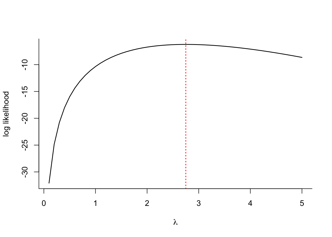
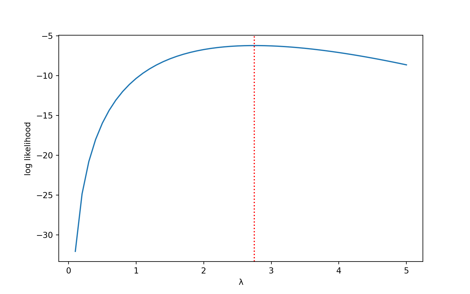
Maximum likelihood estimation (MLE) is an intuitive and important estimation principle in statistics. It is based on the distributional properties of the data, hence it applies to stochastic data modeling. If the observed data \(\textbf{y}\) are the realization of a data-generating random mechanism, then it makes sense to examine the probability distribution of the data and choose as parameter estimates those values that make it most likely to have observed the data. In other words, we use the probability distribution to find the most likely explanation for the data—hence the name maximum likelihood.
Making progress with MLE requires that we know the joint distribution of the random vector \(\textbf{Y}\), an \(n\)-dimensional distribution. The distribution depends on a vector \(\boldsymbol{\theta}\) of unknown parameters and we denote it as \(f(\textbf{y}; \boldsymbol{\theta})\).
When the observations are independent, the joint density is the product of the individual densities, \[
f(\textbf{y}; \boldsymbol{\theta}) = \prod_{i=1}^n \, f(y_i; \boldsymbol{\theta})
\]
Invariance
Maximum likelihood estimation is popular because it is an intuitive principle if we accept a random data-generating mechanism. MLEs have very appealing properties, for example, they are invariant estimators. If \(\widehat{\theta}\) is the MLE of \(\theta\), then \(g(\widehat{\theta})\) is the maximum likelihood estimator of \(g(\theta)\).
In generalized linear models, a linear predictor is related to a transformation of the mean through the link function \[
g(\mu) = \eta = \beta_0 + \beta_1x_1 + \cdots + \beta_p x_p
\] For example, if the data are Poisson random variables, \(g(\cdot)\) is typically the log function (the log link). The coefficient estimates have a linear interpretation on the logarithmic scale. Suppose \(\boldsymbol{\beta}\) is estimated by maximum likelihood and is used to construct a 95% confidence interval \([\widehat{\eta}_{.025},\widehat{\eta}_{.975}]\) for \(\eta\).
You can transform from \(\eta\) to \(\mu\) by inverting the link function, \(\mu = g^{-1}(\mu)\). Thus, \[
\left[ \exp\{\widehat{\eta}_{.025}\}, \exp\{\widehat{\eta}_{.975}\} \right]
\] is a 95% confidence interval for \(\mu\).
In Section 60.4.2 we discussed calculating a confidence interval for the event probability of a Bernoulli(\(\pi\)) distribution based on the Central Limit Theorem. The interval we derived was \[
\widehat{\pi} \pm \frac{z_{1-\alpha/2}}{\sqrt{n}}\sqrt{\widehat{\pi}(1-\widehat{\pi})}
\] and it is not guaranteed to fall between 0 and 1. While \(\widehat{\pi}\) is between 0 and 1, adding and subtracting from it might push the confidence bounds beyond the permissible range.
An MLE-based confidence interval that obeys the (0,1) boundaries can be constructed based on the simple logistic regression model \[
\log\left( \frac{\pi}{1-\pi} \right ) = \beta_0
\]
The MLE of \(\widehat{\pi}\) is \(\overline{y}\), and the estimate of \(\beta_0\) is thus \[
\widehat{\beta}_0 = \log\left( \frac{\overline{y}}{1-\overline{y}} \right )
\] A \((1-\alpha) \times 100\%\) confidence interval for \(\beta_0\), based on the asymptotic Gaussian distribution of the maximum likelihood estimator, is \[
\left[\widehat{\beta}_0 - z_{\alpha/2}\,\text{se}(\widehat{\beta}_0), \quad \widehat{\beta}_0 + z_{\alpha/2}\,\text{se}(\widehat{\beta}_0)
\right] = [\widehat{\eta}_{\alpha/2}, \widehat{\eta}_{1-\alpha/2}]
\] where \(\text{se}(\widehat{\beta}_0)\) is the standard error of the intercept. Plug these \((1-\alpha) \times 100\%\) confidence bounds for \(\beta_0\) into the inverse of the logit transform and you get \((1-\alpha) \times 100\%\) confidence bounds for \(\pi\): \[
\left[\frac{1}{1+\exp\{-\widehat{\eta}_{\alpha/2}\}}, \quad \frac{1}{1+\exp\{-\widehat{\eta}_{1-\alpha/2}\}}\right]
\]
For a finite sample size, MLEs are not necessarily optimal estimators but they have appealing properties as the sample size grows. As \(n \rightarrow \infty\), maximum likelihood estimators
- are consistent, that means they converge in probability to the true value
- are normally distributed
- are efficient in that no other estimator has an asymptotically smaller mean squared error
Linear Model with Gaussian Errors
Suppose we want to find an estimator for \(\boldsymbol{\beta}\) in the linear model \(\textbf{Y} = \textbf{X}\boldsymbol{\beta} + \boldsymbol{\epsilon}\), where the model errors follow a Gaussian distribution with mean \(\textbf{0}\) and variance \(\textbf{V}\). \(\textbf{Y}\) then follows a Gaussian distribution because it is a linear function of \(\boldsymbol{\epsilon}\) (see Section 61.10). The probability density function of \(\textbf{Y}\) is
\[
f\left( \textbf{Y} \right)=\frac{\left| \textbf{V} \right|^{- 1/2}}{(2\pi)^{\frac{n}{2}}}\exp\left\{ - \frac{1}{2}\left( \textbf{Y} - \textbf{X}\boldsymbol{\beta} \right)^\prime\textbf{V}^{- 1}\left( \textbf{Y} - \textbf{X}\boldsymbol{\beta} \right) \right\}
\]
This joint distribution of the data can be used to derive the maximum likelihood estimator (MLE) of \(\boldsymbol{\beta}\). Maximum likelihood estimation considers this as a function of \(\boldsymbol{\beta}\) rather than a function of \(\textbf{Y}.\) Maximizing this likelihood function \(\mathcal{l}(\boldsymbol{\beta};\textbf{Y})\) is equivalent to maximizing its logarithm. The log-likelihood function for this problem is given by
\[
\ln\mathcal{l}\left( \boldsymbol{\beta};\textbf{Y} \right\} = l\left( \boldsymbol{\beta};\textbf{Y} \right) = - \frac{1}{2}\ln\left( \left| \textbf{V} \right| \right) - \frac{n}{2}\ln(2\pi) - \frac{1}{2}\left( \textbf{Y} - \textbf{X}\boldsymbol{\beta} \right)^\prime\textbf{V}^{- 1}\left( \textbf{Y} - \textbf{X}\boldsymbol{\beta} \right)
\]
Finding the maximum of this function with respect to \(\boldsymbol{\beta}\) is equivalent to minimizing the quadratic form \[
\left( \textbf{Y} - \textbf{X}\boldsymbol{\beta} \right)^\prime\textbf{V}^{-1}\left( \textbf{Y} - \textbf{X}\boldsymbol{\beta} \right)
\] with respect to \(\boldsymbol{\beta}\). Applying the results about matrix differentiation in Section 61.9 leads to
\[\begin{align*}
\frac{\partial}{\partial\boldsymbol{\beta}}\left( \textbf{Y} - \textbf{X}\boldsymbol{\beta} \right)^\prime\textbf{V}^{- 1}\left( \textbf{Y} - \textbf{X}\boldsymbol{\beta} \right) &= \frac{\partial}{\partial\boldsymbol{\beta}}\left\{ \textbf{Y}^\prime\textbf{V}^{- 1}\textbf{Y} - 2\textbf{Y}^\prime\textbf{V}^{- 1}\textbf{X}\boldsymbol{\beta} + \boldsymbol{\beta}^\prime\textbf{X}^\prime\textbf{V}^{- 1}\textbf{X}\boldsymbol{\beta} \right\} \\
&= - 2\textbf{X}^\prime\textbf{V}^{- 1}\textbf{Y} + 2\textbf{X}^\prime\textbf{V}^{- 1}\textbf{X}\boldsymbol{\beta}
\end{align*}\]
The derivative is zero when \(\textbf{X}^\prime\textbf{V}^{- 1}\textbf{Y} = \textbf{X}^\prime\textbf{V}^{- 1}\textbf{X}\boldsymbol{\beta}\).
If \(\textbf{X}\) is of full column rank, then \(\textbf{X}^\prime\textbf{V}^{- 1}\textbf{X}\) is non-singular and its inverse exists. Pre-multiplying both sides of the equation with that inverse yields the solution
\[\begin{align*}
\textbf{X}^\prime\textbf{V}^{- 1}\textbf{Y} &= \textbf{X}^\prime\textbf{V}^{- 1}\textbf{X}\widehat{\boldsymbol{\beta}} \\
\left( \textbf{X}^{\prime}\textbf{V}^{- 1}\textbf{X} \right)^{- 1}\textbf{X}^\prime\textbf{V}^{- 1}\textbf{Y} &= {\left( \textbf{X}^{\prime}\textbf{V}^{- 1}\textbf{X} \right)^{- 1}\textbf{X}}^\prime\textbf{V}^{- 1}\textbf{X}\widehat{\boldsymbol{\beta}} \\
\left( \textbf{X}^{\prime}\textbf{V}^{- 1}\textbf{X} \right)^{- 1}\textbf{X}^\prime\textbf{V}^{- 1}\textbf{Y} &= \widehat{\boldsymbol{\beta}}
\end{align*}\]
The maximum likelihood estimator of \(\boldsymbol{\beta}\) is the generalized least squares estimator
\[\widehat{\boldsymbol{\beta}}_{GLS} = \left( \textbf{X}^{\prime}\textbf{V}^{- 1}\textbf{X} \right)^{- 1}\textbf{X}^\prime\textbf{V}^{- 1}\textbf{Y}\]
A special case arises when the model errors \(\boldsymbol{\epsilon}\) are uncorrelated and the variance matrix \(\textbf{V}\) is a diagonal matrix:
\[
\textbf{V} = \begin{bmatrix}
\sigma_{1}^{2} & \cdots & 0 \\
\vdots & \ddots & \vdots \\
0 & \cdots & \sigma_{n}^{2}
\end{bmatrix}
\]
Since the errors are Gaussian distributed, we know that the errors are then independent. The MLE of \(\boldsymbol{\beta}\) is the weighted least squares estimator
\[
\widehat{\boldsymbol{\beta}}_{WLS} = \left(\textbf{X}^\prime\textbf{W}\textbf{X}\right)^{-1}\textbf{X}^\prime\textbf{W}\textbf{Y}
\] where \(\textbf{W} = \textbf{V}^{-1}\).
A further special case arises when the diagonal entries are all the same,
\[\textbf{V} = \begin{bmatrix}
\sigma^{2}\ & \cdots & 0 \\
\vdots & \ddots & \vdots \\
0 & \cdots & \sigma^{2}
\end{bmatrix} = \sigma^{2}\textbf{I}\]
We can write the error distribution in this case as \(\boldsymbol{\epsilon} \sim G\left(\textbf{0},\sigma^{2}\textbf{I} \right)\) and the model for \(\textbf{Y}\) as \(\textbf{Y} \sim G\left( \textbf{X}\boldsymbol{\beta},\sigma^{2}\textbf{I} \right)\).
Under this iid assumption for the Gaussian linear model we can substitute \(\sigma^{2}\textbf{I}\) for \(\textbf{V}\) in the formula for \(\widehat{\boldsymbol{\beta}}\). The maximum likelihood estimator for \(\boldsymbol{\beta}\) is the ordinary least squares estimator:
\[\widehat{\boldsymbol{\beta}}_{OLS} = \left( \textbf{X}^{\prime}\textbf{X} \right)^{- 1}\textbf{X}^\prime\textbf{Y}\]
Notice that \(\sigma^{2}\) cancels out of the formula; the value of the OLS estimator does not depend on the inherent variability of the data. However, the variability of the OLS estimator does depend on \(\sigma^{2}\) (and on \(\textbf{X}\)).
Now that we have found the MLE of \(\boldsymbol{\beta}\), the parameters in the mean function, we can also derive the MLE of the parameters in the variance-covariance structure of the multi-variate Gaussian. Let’s do this for the iid case, \(\boldsymbol{\epsilon} \sim G(\textbf{0},\sigma^2\textbf{I})\). The joint density of the data can then be written as \[
f(\textbf{Y}) = \prod_{i=1}^n (2 \pi\sigma^2)^{-1/2} \exp\left\{-\frac{1}{2\sigma^2} (y_i - \textbf{x}_i^\prime\boldsymbol{\beta})^2\right\}
\] Taking logs and arranging terms, the log-likelihood function for \(\sigma^2\) is \[
\mathcal{l}(\sigma^2; \textbf{y}) = -\frac{n}{2}\log(2\pi\sigma^2) -\frac{1}{2\sigma^2}\sum_{i=1}^n(y_i - \textbf{x}_i\prime\boldsymbol{\beta})^2
\]
Taking the derivative of \(\mathcal{l}(\sigma^2; \textbf{y})\) with respect to \(\sigma^2\), setting it to zero and arranging terms results in \[
\frac{1}{\sigma^4}\sum_{i=1}^n(y_i - \textbf{x}_i^\prime\boldsymbol{\beta})^2 = \frac{n}{\sigma^2}
\] The MLE of \(\sigma^2\) in this case is \[
\widehat{\sigma}^2 = \frac{1}{n}\sum_{i=1}^n(y_i - \textbf{x}_i^\prime\boldsymbol{\beta})^2
\] The MLE of \(\sigma^2\) looks similar to the estimator we used in the OLS case, \[
\frac{1}{n-r(\textbf{X})} \sum_{i=1}^n(y_i - \textbf{x}_i^\prime \widehat{\boldsymbol{\beta}})^2 = \frac{1}{n-r(\textbf{X})} \, \text{SSE}
\] with two important differences. The divisor in the MLE is \(n\) instead of \(n-r(\textbf{X})\) and the MLE uses \(\boldsymbol{\beta}\) rather than the OLS estimator \(\widehat{\boldsymbol{\beta}}\) in the sum-of-squares term. In practice, we would substitute the MLE for \(\boldsymbol{\beta}\) to compute \(\widehat{\sigma}^2\), so that the least squares-based estimator and the maximum likelihood estimator differ only in the divisor. Consequently, they cannot be both unbiased estimators of \(\sigma^2\). Which should we choose?
We can think of the divisor \(n-r(\textbf{X})\) as accounting for the actual degrees of freedom, the amount of information if you will, in the estimator. Since we are using an estimate of \(\boldsymbol{\beta}\) to compute SSE, we have “used up” information in the amount of the rank of \(\textbf{X}\). This is the same rationale that computes the estimate of the sample variance as \[
s^2 = \frac{1}{n-1} \sum_{i=1}^n \left(y_i - \overline{y}\right)^2
\] because we are using the sample mean \(\overline{y}\) in the computation rather than the true mean. Once the sample mean is known, only \((n-1)\) of the \(y_i\) can be chosen freely, the value of the last one is determined.
The reason the MLE divides by \(n\) instead of \(n-r(\textbf{X})\) is that it uses \(\boldsymbol{\beta}\) and does not need to account for information already “used up” in the estimation of the mean function. If you substitute \(\widehat{\boldsymbol{\beta}}\) for \(\boldsymbol{\beta}\), the MLE of \(\sigma^2\) is a biased estimator.

