23 General Concepts
Quotes
We love to predict things—and we aren’t very good at it.
It is difficult to predict, especially the future.
23.1 Signal and Noise
The signal represents the systematic, non-random effects in the data. The noise is the unpredictable, unstructured and non-systematic, randomness around the signal.
A slightly different, and also useful, definition of noise stems from intelligence analysis. The signal is the information we are trying to find, the noise is the cacophony of other information that obscures the signal. That information might well be a signal for something else but it is irrelevant or useless for the event the intelligence analyst is trying to predict.
Information not being relevant for the signal we are trying to find is the key. In the view of the data scientist, that information is due to random events.
Finding the signal is not trivial, different analysts can arrive at different models to capture it. Signals can be obscured by noise. Multiple signals can hide in the data, for example, short-term and long-term cyclical trends in time series data. What appears to be a signal might just be random noise that we mistake for a systematic effect.
Example: Theophylline Concentration
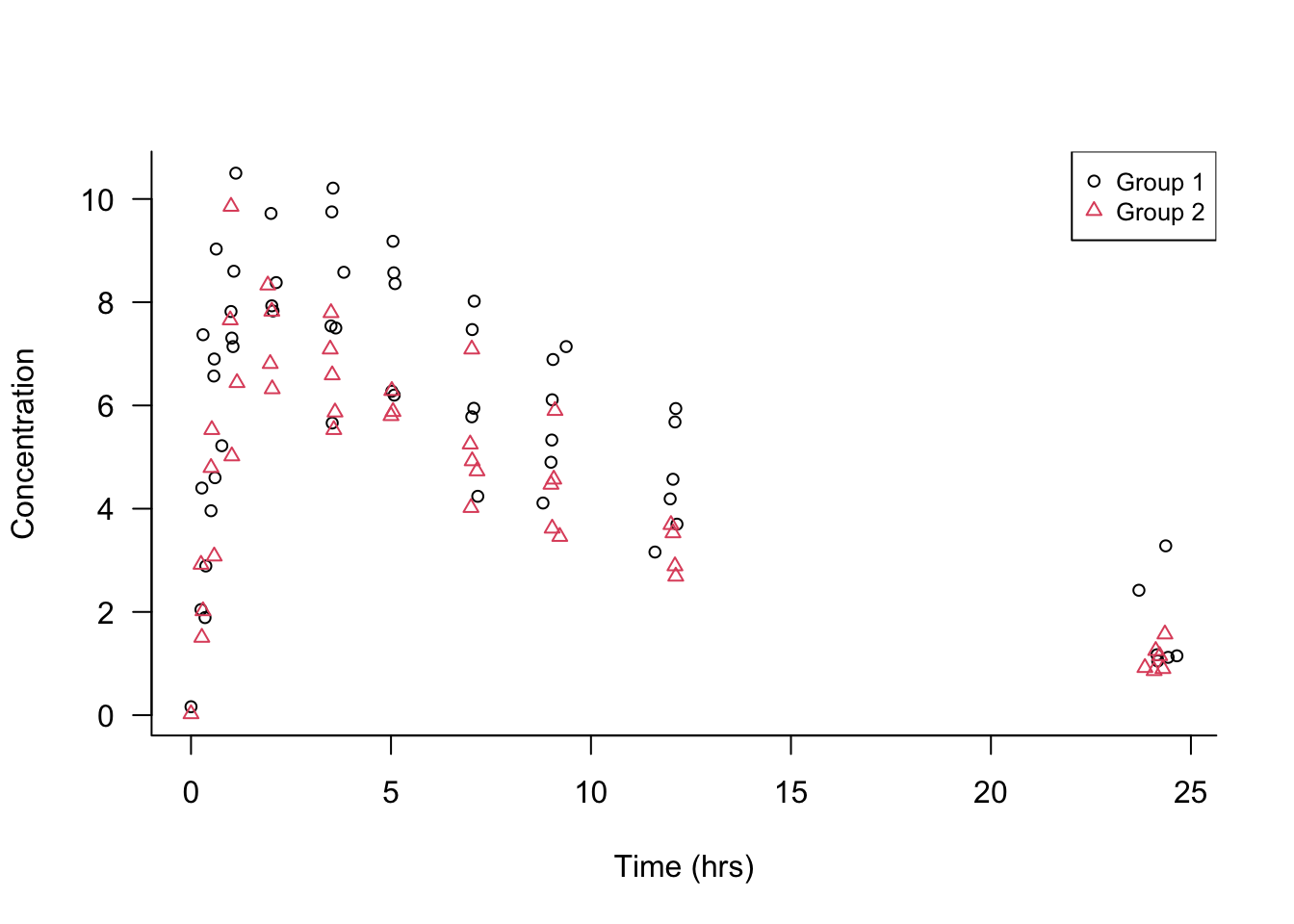
Figure 23.1 shows the concentration of the drug theophylline over 24 hours after administration of the drug in two groups of patients. There are 98 data points of theophylline concentration and measurement time. What are the signals in the data? What is noise?
The first observation is that the data points are not all the same over time, otherwise they would fall on a horizontal straight line: there is variability in the data. Separating signal and noise means attributing this variability to different sources: some systematic, some random.
Focusing on either the open circles (group 1) or the triangles (group 2), you notice that points that are close in time are not necessarily close in the concentration measurement. Not all patients were measured at exactly the same time points, but at very similar time points. For example, concentrations were measured after about 7, 9, and 12 hours. The differences in the concentration measurements among the patients receiving the same dosage might be due to patient-to-patient variability or measurement error.
Focusing on the general patterns of open circles and triangles, it seems that the triangles appear on average below the average circle a few hours after administration. Absorption of theophylline into the body and elimination from the body appear to be different in the two groups.
Much of the variability in the data seems to be a function of time. Shortly after administering the drug the concentration rises, reaches a maximum level, and declines as the drug is eliminated from the body. Note that this sentence describes a general overall trend in the data.
Which of these sources of variability are systematic—the signals in the data— and which are random noise?
Patient-to-patient variability within a group at the same time of measurement: we attribute this to random variation among the participants.
Possible measurement errors in determining the concentrations: random noise
Overall trend of drug concentration over time: signal
Differences among the groups: signal
These assignments to signal and noise can be argued. For example, we might want to test the very hypothesis that there are no group-to-group differences. If that hypothesis is true, any differences between the groups we discern in Figure 23.1 would be due to chance; random noise in other words.
The variability between patients could be due to factors such as age, gender, medical condition, etc. We do not have any data about these attributes. By treating these influences as noise, we are making important assumptions that their effects are irrelevant for conclusions derived from the data. Suppose that the groups refer to smokers and non-smokers but also that group 1 consists of mostly men and group 2 consists of mostly women. If we find differences in theophylline concentration over time among the groups, we could not attribute those to either smoking status or gender.
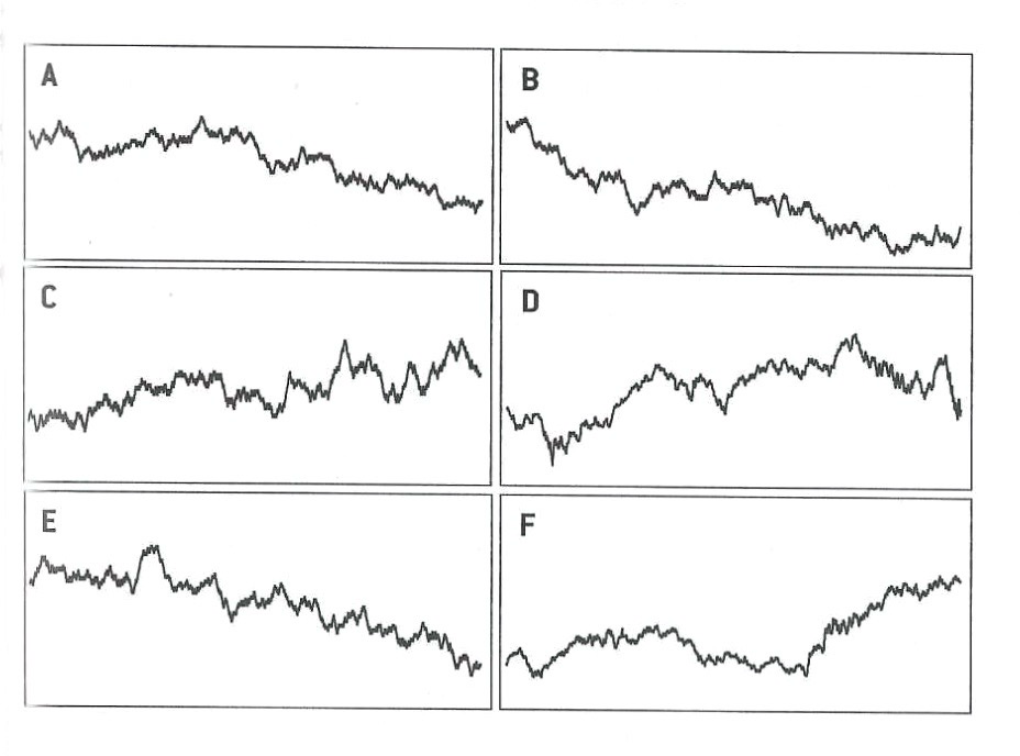
Finding the signal in noisy data is not trivial. The opposite can also be difficult: not mistaking noise for a signal. Figure 23.2 is taken from Silver (2012, 341) and displays six “trends”. Four of them are simple random walks, the result of pure randomness. Two panels show the movement of the Dow Jones Industrial Average (DJIA) during the first 1,000 trading days of the 1970s and 1980s. Which of the panels are showing the DJIA and which are random noise?
What do we learn from this?
Even purely random data can appear non-random over shorter sequences. We can easily fall into the trap of seeing a pattern (a signal) where there is none. Sometimes there is no signal at all. After drawing two unlikely poker hands in a row there is not a greater chance of a third unlikely hand unless there is some systematic effect (cards not properly shuffled, game rigged). Our brains ignore that fact and believe that we are more lucky than is expected by chance. Paul the Octopus predicted the winner of 12 out of 14 soccer matches correctly; I would argue purely by chance.
Data that contains clear long-run signals—the stock market value is increasing over time—can appear quite random on shorter sequences. One a day-to-day basis predicting whether the market goes up or down is very difficult. In the long run ups and downs are almost equally likely. Upswings have a slight upper hand and are on average greater than the downswings, increasing the overall value in the long term. Traders who try to beat the market over the short run have their work cut out for them.
By the way, panels D and F in Figure 23.2 are from actual stock market data. Panels A, B, C, and E are pure random walks. It would not be surprising if some investors would bet money on “trend” C.
23.2 Types of Statistical Learning
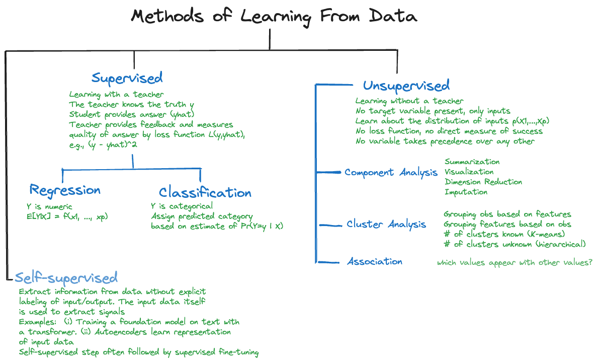
The primary distinction of learning methods in data science is between supervised and unsupervised methods of learning (Figure 23.3). However, there are other important forms of learning from data, for example, self-supervised learning, active learning, and reinforcement learning (RL), which are important for machine learning and artificial intelligence applications.
Supervised Learning
Definition: Supervised Learning
Supervised learning trains statistical learning models through a target variable.
Supervised learning is characterized by the presence of a target variable (dependent variable, response variable, output variable); it is the attribute about which we want to draw inferences (predict, classify, estimate. test hypotheses). The training and test data sets contain values for the target variable, also called the labels in machine learning. Data for supervised learning is often called labeled data (see Figure 23.3). The other variables in the data set are potentially input variables. Other commonly used names for the inputs are independent variables, predictor variables, regression variables. Supervised learning is the predominant form of learning in data science applications.
Goals of supervised learning include to
- Predict the target variable from input variables.
- Classify observations into categories of the target variable based on the input variables.
- Develop a function that approximates the underlying relationship between inputs and outputs.
- Understand the relationship between inputs and outputs.
- Group observations into sets of similar data based on the values of the target variable and based on values of the inputs.
- Reduce the dimensionality of the problem by transforming target and inputs from a high-dimensional to a lower-dimensional space.
- Test hypotheses about the target variable.
Studies can pursue one or more of these goals. For example, you might be interested in understanding the relationship between target and input variables and use that relationship to predict and to test hypotheses.
The name supervised learning comes from thinking of learning in an environment that is supervised by a teacher. The teacher asks questions for which they know the correct answer (the ground truth) and judge a student’s response to the questions. The goal is to increase students’ knowledge as measured by the quality of their answers. But we do not want students to just memorize answers, we want to teach them to be problem solvers, to apply the knowledge to new problems, to be able to generalize.
The parallel between the description of supervised learning in a classroom and training an algorithm on data is obvious: the problems asked by the teacher, the learning algorithm, are the data points, the target \(Y\) is the correct answer, the inputs \(x_{1},\cdots,x_{p}\) are the information used by the students to answer the question. The discrepancy between question and answer is measured by a loss function: \[ (y - \widehat{y})^2 = (y - \widehat{f}\left( x_{1},\cdots x_{p} \right))^2 \] or some such metric. Teaching the students reduces the loss as their answers get closer to the correct answers, the ground truth. Training stops when the students can transfer knowledge to solve previously unseen problems. We are not interested in teaching students to memorize the answers to the questions asked in class. If that were the case we would just train until the loss function reaches zero on the training data. We would not know whether the students have learned the concepts or just memorized the answers. To avoid the latter, we need to validate the students’ knowledge on new questions and not overdo memorization.
Table 23.1 contains a non-exhaustive list of algorithms and models you encounter in supervised learning.
| Linear regression | Nonlinear regression | Regularized regression (Lasso, Ridge, Elastic nets) |
| Local polynomial regression (LOESS) | Smoothing splines | Kernel regression. |
| Logistic regression (binary & binomial) | Multinomial regression (nominal and ordinal) | Poisson regression (counts and rates) |
| Decision trees | Random forests | Bagged trees |
| Adaptive boosting | Gradient boosting machine | Extreme gradient boosting |
| Naïve Bayes classifier | Nearest-neighbor methods | Discriminant analysis (linear and quadratic) |
| Principal component regression | Partial least squares | Generalized linear models |
| Generalized additive models | Mixed models (linear and nonlinear) | Models for correlated data (spatial, time series) |
| Support vector machines | Neural networks | Extreme gradient boosting |
There is a lot to choose from, and for good reason. The predominant application of data analytics is supervised learning with batch (or mini-batch) data. In batch data analysis the data already exist as a historical data source in one place. We can read all records at once or in segments (called mini-batches). If we have to read the data multiple times, for example, because an iterative algorithm passes through the data at each iteration, we can do so.
Unsupervised Learning
Definition: Unsupervised Learning
In unsupervised learning methods a target variable is not present.
Unsupervised learning does not utilize a target variable; hence it cannot predict or classify observations in the usual sense. However, we are still interested in discovering structure, patterns, and relationships in the data. When data are grouped into sets of similar data points by an unsupervised algorithm, we might want to predict which group a new observation belongs to. This sounds like a prediction in a classification model. The difference is that in a supervised context we know the class memberships during training. In an unsupervised context the definition of the classes (the clusters) is the output of the learning method.
The term unsupervised refers to the fact that we no longer know the ground truth because there is no target variable. The concept of a teacher who knows the correct answers and supervises the learning progress of the student does not apply. In unsupervised learning there are no clear error metrics by which to judge the quality of an analysis, which explains the proliferation of unsupervised methods and the reliance on heuristics. For example, a 5-means cluster analysis will find five groups of observations in the data, whether this is the correct number or not, and it is up to us to interpret what differentiates the groups and to assign group labels.
Often, unsupervised learning is used in an exploratory fashion, improving our understanding of the joint distributional properties of the data and the relationships in the data. The findings then help lead us toward supervised approaches.
A coarse categorization of unsupervised learning techniques also hints at their application:
Association analysis: which values of the variables \(x_{1},\cdots,x_{p}\) tend to occur together in the data? An application is market basket analysis, where the \(X\)s are items are in a shopping cart (or a basket in the market), and \(x_{i} = 1\) if the \(i\)th item is present in the basket and \(x_{i} = 0\) if the item is absent. If items frequently appear together, bread and butter, or beer and chips, for example, then maybe they should be located close together in the store. Association analysis is also useful to build recommender systems: shoppers who bought this item also bought the following items
Cluster analysis: can data be grouped based on \(x_{1},\cdots,x_{p}\) into sets such that the observations within a set are more similar to each other than they are to observations in other sets? Applications of clustering include grouping customers into segments. Segmentation analysis is behind loyalty programs, lower APRs for customers with good credit rating, and churn models.
Dimension reduction: can we transform the inputs \(x_{1},\cdots,x_{p}\) into a set \(c_{1},\cdots,c_{k}\), where \(k \ll p\) without losing relevant information? Applications of dimension reduction are in high-dimensional problems where the number of inputs is large relative to the number of observations. In problems with wide data, the number of inputs \(p\) can be much larger than \(n\), which eliminates many traditional methods of analysis from consideration.
Anomaly (Outlier) detection: can we identify unusual observations or patterns in the data.
Methods of unsupervised learning often precede supervised learning; the output of an unsupervised learning method can serve as the input to a supervised method. An example is dimension reduction through principal component analysis (PCA) prior to supervised regression. Suppose you have \(n\) observations on a target variable \(Y\) and a large number of potential inputs \(x_{1},\cdots,x_{p}\) where \(p\) is large relative to \(n\). PCA computes linear combinations of the \(p\) inputs that account for decreasing amounts of variability among the \(X\)s. These linear combinations are called the principal components. For example, the first principal component explains 70% of the variability in the inputs, the second principal component explains 20% and the third principal component 5%. Rather than building a regression model with \(p\) predictors, we use only the first three principal components as inputs in the regression model. The resulting regression model is called a principal component regression (PCR) because its inputs are the result of a PCA. The PCA is an unsupervised model because it does not use information about \(Y\) in forming the principal components. If \(p = 250\), using the first three principal components replaces
\[ Y = \beta_{0} + \beta_{1}{\ x}_{1} + \beta_{2}x_{2} + \beta_{3}x_{3} + \beta_{4}x_{4} + \cdots + \beta_{250}x_{250} + \epsilon \] with \[ Y = \alpha_{0} + \alpha_{1}c_{1} + \alpha_{2}c_{2} + \alpha_{3}c_{3} + \epsilon \]
where \(c_{1}\) denotes the first principal component, itself a linear combination of the 250 inputs
\[ c_{1} = \gamma_{1}x_{1} + \gamma_{2}x_{2} + \gamma_{3}x_{3} + \cdots + \gamma_{250}x_{250} \]
Self-supervised Learning
Self-supervised learning (SSL) is a form of learning that combines elements of supervised and unsupervised learning. Like unsupervised learning, the data is not labeled, that is, there is no target variable. Like the majority of supervised learning applications, the goal is to predict or classify.
SSL accomplishes these seemingly contradictory features by implicitly and autonomously extracting relationships, patterns, and knowledge from the training data. It creates its own supervisory signals from unlabeled data; the model learns to predict parts of its input from other parts. For example, a language model trained on text can predict more text.
Transformer models such as GPTs (generative pretrained transformers), are trained in a self-supervised way as autoregressive language model. During training the model learns the relevant patterns and relationships in the text input data.
In a second step, applications are built on top of the foundation models trained in a self-supervised fashion. For example, ChatGPT is a question-answer applications built on top of the GPT foundation model.
Active Learning
Active learning is another technique to make use of limited amounts of labeled data. Consider the situation where some data are labeled and some data are not yet labeled. This situation can arise when creating the labels is done by human interpreters and is time consuming (labeling images, extracting information from video or audio data, …).
An active learning algorithm begins training on the available labeled data and strategically suggests which of the unlabeled data to best add to the training set. Human interpreters then label the suggested data and add it to the training data. The model is then retrained on the enlarged data set.
The key distinction between self-supervised and active learning is that SSL creates its own labels from unlabeled data, while active learning intelligently requests human-provided labels for specific examples.
Reinforcement Learning
Reinforcement learning (RL) is unique to machine learning and does not fall neatly in the supervised/unsupervised learning categories. It is a powerful method that received much attention when algorithms were trained on data to play games.
In reinforcement learning, an agent (a player) is taking actions (makes moves) in an environment (the game). The agent learns by interacting with the environment by receiving feedback on the moves. Actions are judged by a reward function (a score) and the system is trained to maximize the sum of future rewards. In other words, given your current position in the game, choose the next move to maximize the score from here on out.
Training computers to play games based on reinforcement learning is fundamentally different from the expert system-based approach that had been used previously. An expert system translates the rules of the game into machine code and adds game strategy. For example, the Stockfish open-source chess program, released first in 2008, has developed with community support into (one of) the best chess engines in the world. In 2017, Google’s DeepMind released AlphaZero, a chess system trained using reinforcement learning. After only 24 hours of training, the data-driven AlphaZero algorithm crushed Stockfish, the best chess engine humans have been able to build over 10 years.
Previously, Google’s DeepMind had developed AlphaGo, a reinforcement-trained system that beat the best Go player in the world, Lee Sedol, four to one. This was a remarkable achievement as Go had been thought to be so complex and requiring intuition that would escape computerization at the level of expert players.
An interesting difference between AlphaGo and AlphaZero is the nature of the training data. Both systems are trained using reinforcement learning. AlphaGo was trained on many records of expert-level games. It was trained to play against historic experts. Success was getting better compared to how human experts played. AlphaZero was trained by playing against itself. Success was beating its former self.
Unlike supervised learning, inputs and outputs do not need to be present in reinforcement learning. The technique is commonly used in robotics, gaming, and recommendation systems.
In 2017, when AlphaGo beat Lee Sedol, it was thought that reinforcement learning would change the world. Despite its remarkable achievement in gameplay and robotics, the impact of RL fell short of expectations.

Why does Reinforcement Learning sometimes fall short? Developing and training reinforcement learning models is an expensive undertaking. The barrier to entry is very high, limiting RL research and development to large tech-savvy organizations. The main reason is the Sim2Real problem mentioned in the tweet above. Reinforcement learning trains an agent in a simulated, artificial environment. The real world is much more complex and transferring training based on simulation to reality is difficult. The RL agents end up performing poorly in real applications.
Until recently, a limitation of RL was the need for a good reward function. It is important that actions in the environment are properly judged. In situations where the result of a move is difficult to judge, reinforcement learning was difficult to apply. For example, in natural language processing, where an action produces some prose, how do we rate the quality of the answer?
This was the problem faced by systems like ChatGPT. How do you score the answer produced during training to make sure the algorithm continuously improves? The solution was a form of reinforcement learning modified by human intervention. RLHF, reinforcement learning with human feedback, uses human interpreters to assign scores to the actions (the ChatGPT answers).
23.3 Regression and Classification
The term regression was coined by Sir Francis Galton in 1877 in his study of genetics. Galton observed a relationship between physical attributes of offspring and their parents. He found that offspring deviated less from the mean value of the population than their parents did. Taller parents tend to have taller children, but children of taller parents tend to be shorter than their parents and children of shorter parents tend to be taller than their parents.
Regression to the Mean
The cause Galton attributed to this phenomenon—which he called regression toward mediocrity—is controversial, his arguments had implications about natural selection and eugenics. As a statistical phenomenon, it is well understood. Attributes are distributed randomly; if you draw an extreme observation from a symmetric distribution, then a subsequent draw is likely to be less extreme, there is a regression to the mean.
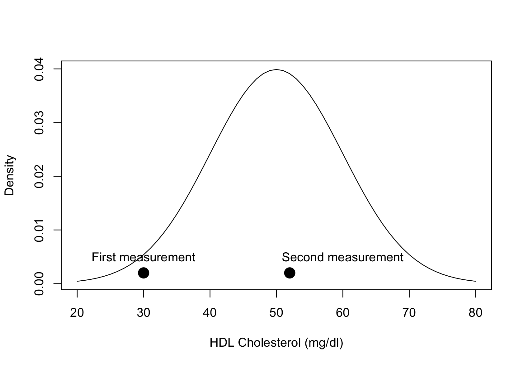
Figure 23.5 displays this phenomenon for the distribution of HDL cholesterol values in a single person. Our cholesterol levels vary from day to day and if their distribution is Gaussian, it might look like the density in the figure, centered at a mean of 50 mg/dl. Suppose you measure a person’s HDL cholesterol, and it results in a first measurement of 30 mg/dl. The value is on the low side of the distribution, but it is not implausible. A follow-up measurement is more likely to be observed near the center of the distribution where most of the probability density is located. A second measurement might thus return a value of 55 mg/dl. A regression to the mean occurred between the first and second measurements.
The regression to the mean phenomenon does not mean regression methods are bad. It is a fact of random variation and a real fallacy when interpreting data. In the cholesterol example, is the change from 30 to 50 mg/dl of HDL due to natural variation or due to a systematic effect, for example, a medical intervention? The regression to the mean fallacy is to misinterpret random variation as a signal.
Example: Testing a Treatment Effect
You want to determine whether a change in diet reduces the risk of heart disease. From a group of individuals, you select those at greatest risk of heart disease and put them on the diet. After some time, you reassess their risk of heart disease.
Because of regression to the mean, the follow-ups will likely show an improvement even if the diet has no effect at all.
The correct way of studying whether the diet has an effect is to randomly divide the individuals into two groups and assign the diet to one group (the treated group) while the other group stays on their normal diet. If the individuals in the treated group improve more than the untreated group, to a degree that cannot be attributed just to chance, then we can make a statement that the diet is effective in reducing the risk of heart disease.
Regression Problems
The term regression has larger meaning today than the regression to the mean phenomenon. Regression problems are those where we study the mean behavior of an attribute and separate it from non-systematic, random behavior.
Definition: Regression Model
A regression model is a statistical model that describes how the mean of a random variable depends on other factors. The factors are often called inputs, predictor variables, independent variables, or regressors.
The variable whose mean is modeled is called the target variable, output variable, response variable, or dependent variable.
Note
It is sometimes assumed that regression models are only for continuous target variables. That is not correct. You can model the mean of a count variable (a discrete variable) or the mean of a categorical variable.
Regression models are not just for continuous response data, they apply to all response types. The defining characteristic is to model the mean as a function of inputs:
\[ \text{E}\lbrack Y\rbrack = f\left( x_{1},\cdots,x_{p},\theta_{1},\cdots,\theta_{k} \right) \]
This expression explicitly lists parameters \(\theta_{1},\cdots,\theta_{k}\) in the mean function. All regression models involve the estimation of unknown, fixed quantities (=parameters). As seen in the non-linear regression example in the introduction, the number of parameters and the number of inputs do not have to be directly related.
Even if the target variable is categorical, we might be interested in modeling the mean of the variable. The simplest case of categorical variables are binary variables with two levels (two categories). This is the domain of logistic regression. As seen earlier, if the categories are coded numerically as \(Y = 1\) for the category of interest (the “event”) and \(Y = 0\) for the “non-event” category, the mean of \(Y\) is a probability. A regression model for a binary target variable is thus a model to predict probabilities. It is sufficient to predict one of the probabilities in the binary context, we call this the event probability \(\pi\). The complement can be obtained by subtraction, \(1 - \pi\).
Extending this principle to more than two categories leads to regression models for multinomial data. If the category variable has \(k\) levels with labels \(C_{1}, \cdots, C_{k}\), we are dealing with \(k\) probabilities; \(\pi_{j}\) is the probability to observe category \(C_{j}\). Suppose that we are collecting data on ice cream preferences on college campuses. A random sample of students are given three ice cream brands in a random order and report the taste as \(C_{1} =\)’yuck’, \(C_{2} =\)’meh’, and \(C_{3} =\)’great’. Modeling these data with regression techniques, we develop a model for the probability to observe category \(j\) as a function of inputs. A multinomial version of logistic regression looks like the following:
\[ \text{Pr}\left( Y = j \right) = \frac{\exp\left\{ \beta_{0j} + \beta_{1j}x_1 + \cdots + \beta_{pj}x_p \right\}} {\sum_{l=1}^k \exp\{\beta_{0l} + \beta_{1l}x_1 + \cdots + \beta_{pl}x_p\}} \]
This is a rather complicated model, but we will see later that it is a straightforward generalization of the two-level case. Instead of one linear predictor we now have separate predictors for the categories. The point of introducing the model here is to show that even in the categorical case we can apply regression methods—they predict category probabilities.
Classification Problems
Classification applies to categorical target variables that take on a discrete number of categories, \(k\). In the binary case \(k = 2\), in the multinomial case \(k > 2\).
The classification problem is to predict not the mean of the variable but to assign a category to an observation. In image classification, for example, an algorithm is trained to assign the objects seen on an image to one of \(k\) possible categories. In the ImageNet competition, \(k=1000\).
The algorithm that maps from input variables to a category is called a classifier. The logic that turns the model output into a category assignment is called the classification rule. Applications of classifications occur in many domains, for example,
- Medical diagnosis: Given a patient’s symptoms, assign a medical condition.
- Financial services: Determine whether a payment transaction is fraudulent.
- Customer intelligence: Assign a new customer to a customer profile (segmentation).
- Computer vision: Detect defective items on an assembly line.
- Computer vision: Identify objects in an image.
- Text classification: Categorize incoming emails as spam.
- Text classification: Categorize the sentiment of a document as positive, neutral, or negative.
- Digital marketing: Predict which advertisement a user is most likely to click.
- Search engine: Given a user’s query and search history predict what link they will follow.
Classification problems can be presented as prediction problems; rather than the mean of a random variable, they predict the membership in a category.
From probabilities to classification
To determine category membership many classification models first go through a predictive step, predicting the probabilities that an observation belongs to the \(k\) categories. The classification rule is then to assign an observation to one category based on the predicted probabilities; usually the category with the highest predicted probability.
Suppose we have a three-category problem with \(\pi_{1} = 0.7,\ \pi_{2} = 0.2,\pi_{3} = 0.1\), and you are asked to predict the category of the next randomly drawn observation. The most likely category to appear is \(C_{1}.\)
This classification rule is known as the Bayes classifier.
Definition: Bayes Classifier
The Bayes classifier assigns an observation with inputs \(x_{1},\cdots,x_{p}\) to the class \(C_{j}\) for which
\[ \Pr(Y = j \, | \, x_{1},\cdots,x_{p}) \]
is largest. The Bayes classifier is optimal in the sense that no other classifier has a smaller mis-classification rate (a greater accuracy).
The Bayes classifier is written as a conditional probability, the probability to observe category \(C_{j}\), given the values of the input variables. The reason for this will become clearer when we cover different methods for estimating category probabilities. Some methods for deriving category probabilities assume that the \(X\)s are random. In regression problems it is assumed that they are fixed, so there is no difference between the unconditional probability \(\Pr\left( Y = j \right)\) and the conditional probability \(\Pr( Y = j \, | \, x_1,\cdots,x_p)\).
We can now see the connection between regression and classification. Develop first a regression model that predicts the category probabilities \(\Pr( Y = j \, | \, x_1,\cdots,x_p)\). Then apply a classification rule to assign a category based on the predicted probabilities. If you side with the Bayes classifier, you choose the category that has the highest predicted probability. For a 2-category problem where events are coded as \(Y=1\) and non-events are coded as \(Y=0\), this means classifying an observation as an event if
\[ \Pr\left( Y = 1\, | \,x_1,\cdots,x_p \right) \geq 0.5 \]
Misclassification rate
While the mean-squared prediction error is the standard measure of model performance in regression models, the performance of a classification model is measured by statistics that contrast the number of correct and incorrect classifications. The most important of these metrics is the misclassification rate (MCR).
Definition: Misclassification Rate
The misclassification rate (MCR) of a classifier is the proportion of observations that are predicted to fall into the wrong category. If \(y_{i}\) is the observed category of the \(i\)th data point, and \({\widehat{y}}_{i}\) is the predicted category, the MCR for a sample of \(n\) observations is
\[ \text{MCR} = \frac{1}{n}\sum_{i = 1}^{n}{I\left( y_{i} \neq {\widehat{y}}_{i} \right)} \]
\(I(x)\) is the indicator function,
\[ I(x) = \left\{ \begin{matrix} 1 & \text{if }x\text{ is true} \\ 0 & \text{otherwise} \end{matrix} \right. \]
The misclassification rate is simply the proportion of observations we predicted incorrectly. Since the target is categorical we do not use differences \(y_i - \widehat{y}_i\) to measure the closeness of target and prediction. Instead, we simply check whether the observed and predicted categories agree (\(y_i = \widehat{y}_i\)). The term \(\sum_{i = 1}^{n}{I\left( y_{i} \neq {\widehat{y}}_{i} \right)}\) counts the number of incorrect predictions. The complement of MCR, the proportion predicted correctly, is called the accuracy of the classification model.
Confusion matrix
The confusion matrix in a classification model with \(k=2\) categories (a binary target) is a 2 x 2 matrix that contrasts the four possibilities of observed and predicted outcomes.
Definition: Confusion Matrix
The confusion matrix in a classification problem is the cross-classification between the observed and the predicted categories. In a problem with two categories, the confusion matrix is a 2 x 2 matrix.
The cells of the matrix contain the number of data points that fall into the cross-classification when the model’s decision rule is applied to \(n\) observations. If one of the categories is labeled positive and the other is labeled negative, the cells give the number of true positive (TP), true negative (TN), false positive (FP), and false negative (FN) predictions.
The following table shows the layout of a typical confusion matrix for a 2-category classification problem. A false positive prediction, for example, is to predict a positive (“Yes”) result when the true state (the observed state) was negative. A false negative result is when the decision rule assigns a “No” to an observation with positive state.
| Observed Category | ||
|---|---|---|
| Predicted Category | Yes (Positive) | No (Negative) |
| Yes (Positive) | True Positive (TP) | False Positive (FP) |
| No (Negative) | False Negative (FN) | True Negative (TN) |
Accuracy of the model is calculated as the proportion of observations that fall on the diagonal of the confusion matrix. The misclassification rate is the complement: the proportion of observations in off-diagonal cells.
Based on the four cells in the confusion matrix many statistics can be calculated (Table 23.3).
| Statistic | Calculation | Notes |
|---|---|---|
| False Positive Rate (FPR) | FP / (FP + TN) | The rate of the true negative cases that were predicted to be positive |
| False Negative Rate (FNR) | FN / (TP + FN) | The rate of the true positive cases that were predicted to be negative |
| Sensitivity | TP / (TP + FN) = 1 – FNR | This is the true positive rate; also called Recall |
| Specificity | TN / (FP + TN) = 1— FPR | This is the true negative rate |
| Accuracy | (TP + TN) / (TP + TN + FP + FN) | Overall proportion of correct classifications |
| Balanced Accuracy | (TP / (TP + FN) + TN / (TN + FP)) / 2 | Average of sensitivity and specificity |
| Misclassification rate | (FP + FN) / (TP + TN + FP + FN) | Overall proportion of incorrect classifications, 1 – Accuracy |
| Precision | TP / (TP + FP) | Ratio of true positives to anything predicted as positive |
| Detection Rate | TP / (TP + TN + FP + FN) | |
| No Information Rate | \(\frac{\max(TP+FN,FP+TN)}{TP+TN+FP+FN}\) | The proportion of observations in the larger observed class |
| F Score | \(\frac{2\text{TP}}{2\text{TP} + \text{FP} + \text{FN}}\) | Harmonic mean of precision and recall |
The model accuracy is measured by the ratio of observations that were correctly classified, the sum of the diagonal cells divided by the total number of observations. The misclassification rate is the complement of the accuracy, the sum of the off-diagonal cells divided by the total number of observations.
The sensitivity (recall) is the ratio of true positives to what should have been predicted as positive. The specificity is the ratio of true negatives to what should have been predicted as negative. These are not complements of each other; they are calculated with different denominators.
One problem with focusing solely on accuracy to measure the quality of a classification model is that the two possible errors, false positives and false negatives might not be of equal consequence. For example, it might not matter how accurate a model is unless it achieves a certain sensitivity—the ability to correctly identify positives.
Consider the data in the Table 23.4, representing 1,000 observations and predictions.
| Observed Category | ||
|---|---|---|
| Predicted Category | Yes (Positive) | No (Negative) |
| Yes (Positive) | 9 | 7 |
| No (Negative) | 26 | 958 |
The classification has an accuracy of 96.7%, which seems impressive. Its false positive and false negative rates are very different, however: FPR = 0.0073, FNR = 0.7429. The model is much less likely to predict a “Yes” when the true state is “No”, than it is to predict a “No” when the true state is “Yes”. Whether we can accept a model with such low sensitivity (100 – 74.29) = 25.71% is questionable, despite the high accuracy. An evaluation of this model should consider whether the two errors, false positive and false negative predictions, are of equal importance and consequence.
It is also noteworthy that the accuracy of 96.7% is not as impressive if you check the no-information rate of the data. The proportion of observations in the larger observed class is (958 + 7)/1,000 = 0.965. The accuracy of the decision rule is only slightly larger. In other words, if you were to take a naïve approach and predict all observations as “No” without looking at the data, that naïve decision rule would have an accuracy of 96.5%. The model did not buy us much over the naïve decision rule.
Accuracy is not a reliable measure when the data are highly unbalanced with respect to the event and non-event categories (see Section 30.3). Unbalanced accuracy, the average of sensitivity and specificity, gives equal weight to the performance on both positive and negative classes, regardless of their proportions in the data set. It prevents the metric from being dominated by the majority class.
The precision of the binary classifier is the number of true positive predictions divided by all positive predictions.
The F-score (also called the \(F_1\) score) is the harmonic mean of precision and recall: \[ F_1 = \frac{2}{\text{Precision}^{-1} + \text{Recall}^{-1}} = \frac{2\text{TP}}{2\text{TP} + \text{FP} + \text{FN}} \] The \(F\) score is popular in natural language applications but is not without problems. The goal of the score is to balance both precision and recall, but the relative importance of the two depends on the problem. The \(F\) score does not take into account true negatives and is problematic if positive and negative outcomes are unbalanced.
Receiver Operator Characteristic (ROC) and Area under the Curve (AUC)
So why do we not build models that have a high accuracy, small false positive rate, and small false negative rate? That seems desirable and we can affect those parameters through the classification rule. To reduce the likelihood of a false positive we could require more evidence before predicting a positive result. Similarly, to reduce the likelihood of false negatives, we could make it more difficult to classify an observation as negative. If \(c\) is the threshold in the decision rule of a binary classification, we could treat it as a parameter and evaluate the performance of the model for different rules
\[ \widehat{\Pr}(Y=1|x_1, \cdots, x_p) > c \] Changing \(c\) affects both false positives and false negatives, as well as the accuracy. For \(c=0.5\) you arrive at the accuracy-optimal Bayes classifier.
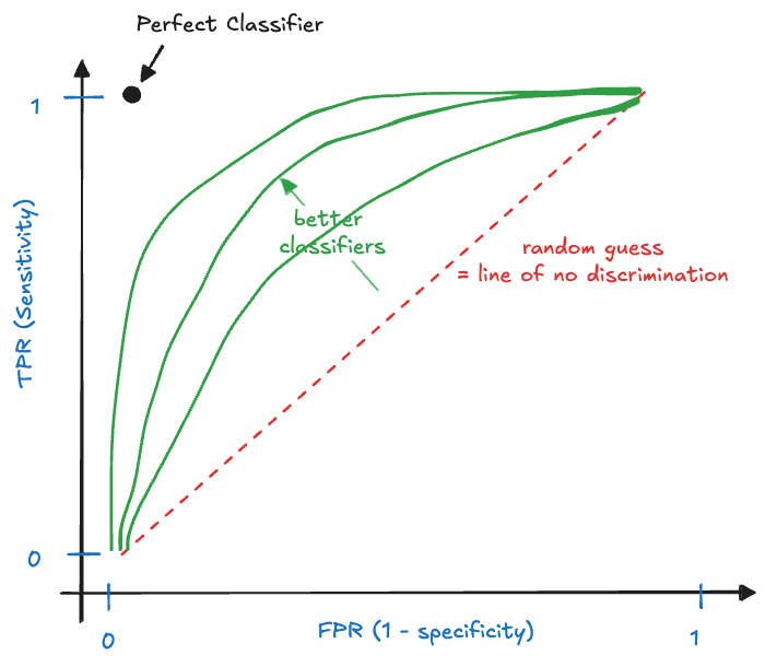
To see how the choice of cutoff affects the performance of a binary classifier, several graphical devices are in use. The receiver operator characteristic (ROC) is a plot of the true positive rate (TPR, sensitivity, recall) against the false positive rate for different values of \(c\). It shows the sensitivity of the classifier as a function of the false positive rate (Figure 23.6).
Tip
The name receiver operator characteristic stems from the method’s origin, it was developed in World War II for operators of military radar receivers to detect enemy objects in battlefields, specifically after the attack on Pearl Harbor in 1941 to measure the operator’s ability to correctly detect Japanese aircraft in radar signals.
A perfect model is one with perfect sensitivity and perfect specificity, it makes no incorrect predictions. It is represented by the point at the (0,1) coordinate in Figure 23.6. The diagonal line represents a random classifier. Suppose you are flipping a coin to predict positive outcomes. The long-run (expected) behavior of this decision rule is captured by the diagonal line. If the coin is fair, you get a point on the line at coordinate (0.5, 0.5). Loaded coins where one side is more likely than the other generate the other points on the 45-degree line.
An actual model will be somewhere between the random classifier and the perfect model. The closer the operating curve is to the left and upper margins of the plot, the more performant the model. Actual ROC curves appear as step functions, after calculating FPR and TPR for a set of threshold values \(c_1, c_2, \cdots\).
The ROC curve shows how sensitivity and specificity change with the threshold value \(c\) and help solve the tradeoff between sensitivity and specificity of the model. The ROC is often summarized by computing AUC, the area under the curve. AUC is a single summary statistic that ranges from 0 to 1, with the uninformative random classifier at AUC = 0.5. The idealistic optimal ROC line that passes through (0, 1) has an AUC of 1. While AUC is a popular summary of a binary classifier, it is not without problems:
Reducing the ROC curve to a single number hides the tradeoffs associated with choosing thresholds; that is the point of the ROC in the first place.
The integration under the ROC curve incorporates extreme ranges of FPR one would usually not consider in real applications. If a false positive rate of more than 80% is unacceptable, why consider such decision rules in evaluating the performance of a model? Typically we are interested in regions of the ROC rather than the entire curve. In screening tests, interest is in the ranges of low FPR, for example. To overcome this issue, partial AUC statistics have been proposed. These restrict FPR, TPR, or both to certain regions of interest.
Precision-Recall Curve
Another graphical display that summarizes the performance of a binary classifier across multiple thresholds is the precision-recall curve (Figure 23.7). Like the ROC, it compares actual classifiers against a no-skill baseline (the horizontal line drawn at the proportion of positives) and an ideal classifier.
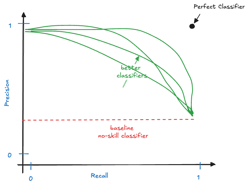
The precision-recall curve can also be summarized by computing the area under its curve (AUC-PR). A large area under the precision-recall curve indicates high precision and high recall of the model across the thresholds. Precision-recall curves are preferred over ROC curves when the data are very imbalanced with respect to positive and negative outcomes.
23.4 Prediction and Explanation
Are we Good at Predicting?
A prediction is a statement about what will happen. In data science, predictions are based on models derived from data.
We predict all the time. On the drive to work we choose this route over that route because we predict it has less traffic, fewer red lights, or we are less likely to get caught behind a school bus. We probably make this choice instinctively, without much deliberation, based on experience, instantaneously processing information about the time of day, weather, etc. An informal model is applied that we have developed based on life experience.
You might choose Netflix over Paramount+ one evening because you think (predict!) it is more likely to deliver content that interests you. This is a prediction problem. You are also on the receiving end of predictions every day. A company offers you a discount because it predicts that without an incentive you might shop at a competitor. We are being served weather forecasts on apps and on the news every day.
We predict all the time; and by many measures we are not very good at it.
In The Signal and the Noise, Silver (2012, 52) cites a study at the University of Pennsylvania that found when political scientists claim that a political outcome had no chance of occurring, it happened about 15% of the time. And of the absolutely sure things they proclaimed, 25% failed to occur. We know that predictions are themselves uncertain, that is why polling results have margins of error. But when you predict that something has a zero chance of happening, then you ought to be pretty confident in that, the margin of error should be small, definitely not 15%.
This is an example of a prediction that is not very good.
If a plane had a 29% of crashing, you would probably consider the risk of flying and stay on the ground. In the run-up to the 2016 presidential election, FiveThirtyEight predicted a 71% chance for Clinton to win the Electoral College and a 29% chance for Trump to win. This was a much higher chance of a Trump victory than the 1% to 15% chance many other models produced. As it turned out, the FiveThirtyEight model was much better than the models that treated the Clinton victory as a near certainty. But both models were wrong about the outcome of the election.
Silver (2012) points out
Most people fail to recognize how much easier it is to understand an event after the fact when you have all the evidence at your disposal. […] But making better first guesses under conditions of uncertainty is an entirely different enterprise than second-guessing.
It is much easier to sift through intelligence after a terrorist attack and to point out what was missed than it is finding the signals in the cacophony of intelligence data before the attack.
Even if our predictions are spot-on, we might not act on them or ignore them. Predictions that contradict our intuition or preferred narrative can be ignored or explained away. Our personal judgment is not as good as you might think. We tend to overvalue our own opinion and this trend increases the more we know. 80% of doctors believe they are in the top 20% of their profession. More than half of them are clearly wrong!
So when a prediction does not come true, does the fault lie with the model of the world or the world itself? If there is a 80% chance of rain tomorrow, then you might see sunny skies. If, in fact, the long run ratio of days that have sunny skies when the forecast calls for an 80% chance of rain is 1 in 5, then the forecast model is correct. We cannot fault the model that calls for a 80% chance of rain for the occasional sunny skies.
Compare this scenario to the following. In the build-up of the the 2008 financial crisis, Standard & Poor gave CDOs, a type of mortgage-backed securities, a stellar AAA credit rating, meaning that there is only a 0.0012 probability that they would fail to pay out over the next 5 years (Silver 2012, 20). In reality, 28% of the AAA-rated CDOs defaulted. Had the world of financial markets drastically changed to bring about such a massive change in default rates (200x!)? Or is it more likely that the default models of the rating agencies were wrong? It was the latter.
Prediction and Forecast
Technically, a prediction and a forecast are different things. In statistics, a prediction results from the application of a model to data. If the data falls outside of the range of observed training data, then it is referred to as a forecast, in particular when the prediction is about a future event.
Forecasting is also referred to as planning in the presence of uncertainty, taking a systematic, methodological approach. Predicting, on the other hand is any proclamation about things we do not know yet. We predict the outcome of a football game based on gut feeling or allegiance to a team, but we forecast the weather based on meteorological models.
In seismology, the distinction between prediction and forecast is taken very seriously. The prediction of an earthquake is a specific statement about when and where it will strike. A forecast, on the other hand, is a statement of probability: there is a 60% chance of an earthquake in Northern Italy over the next fifty years. Leaning on this distinction, the official U.S. Geological Service attitude is that earthquakes cannot be predicted.
With apologies to purists and seismologists, we use the terms predicting and forecasting interchangeably. What matters is that predictions and forecasts in our context are based on modeling data.
Bad Predictions
If we are not good at predicting, can we learn from what bad predictions have in common? Silver (2012, 20) lists some attributes of bad predictions:
- Focus on the signals that tell a story about the world as we would like it to be, not how it really is.
- Ignore the risks that are most difficult to measure, although they pose the greatest risk to our well-being.
- Make approximations and assumptions that are much cruder than we realize.
- Dislike (abhor) uncertainty, even if it is an integral part of the problem.
If we want to avoid these mistakes when modeling data, we need to
- Build models that are useful abstractions, not too complicated and not too simple.
- Find the signal that the data is trying to convey, not the signal we wish or hope to find. And allow for generalization beyond the data at hand.
- Be honest about the quality of the data and the limitations to capture complex systems through quantification.
- Quantify the uncertainty in the conclusions drawn from the model.
Difficult to Predict
This sounds good and is a noble undertaking. Unfortunately, some things are notoriously difficult to predict.
Chaotic systems
like the weather or economy that resist manipulation. Fortunately, we have much experience in predicting the weather, it is a daily exercise with lots of data to fall back on.Noisy systems
are difficult to predict because they have a low signal-to-noise ratio. Data collected in the social sciences often suffers from high variability, humans are a very variable bunch.Complex systems
are those governed by the interaction of many separate individual parts. They can seem at once very predictable and very unpredictable. The laws governing earthquakes are well understood and the long-term frequency of a magnitude 6.5 earthquake in Los Angeles can be estimated well. But we are not very good at predicting earthquake activity. Complex systems periodically undergo violent and highly nonlinear phase changes from orderly to chaotic and back again. Bubbles in the economy and significant weather events such as hurricanes, tornadoes, or tsunamis are examples.Nonlinear growth systems
When growth is linear we have a good handle on describing and modeling change. When growth is nonlinear, for example, exponential, predicting outcomes is much more difficult. Small deviations in the model today translate into massive discrepancies in the future. Infectious diseases are a good example.Feedback systems
In systems with feedback loops the act of predicting can change the system being predicted. Economic predictions can change the way people behave and that can affect the outcome of the prediction itself.
Self-fulfilling predictions, where the prediction reinforces the outcome, are common in political polling. A poll showing a candidate surging can cause voters to switch to the candidate from ideologically similar candidates. Or it can make undecided voters to finally get off the fence.
A self-cancelling prediction works the opposite way, it undermines itself. When GPS systems became more commonplace, drivers were guided to routes which the systems thought had less traffic. If the systems cannot adjust in real time to the actual traffic density, the guidance can result in more traffic on the suggested routes.
An example of a self-fulfilling prediction is when increased media coverage of a medical condition leads to increased diagnosis of the condition. Not just because the condition is more prevalent, but because of increased attention people are more likely to identify symptoms and doctors are more likely to diagnose them. The rise of autism diagnoses in the U.S. from 1992 to 2008 correlates highly with the media coverage of autism (Silver 2012, 218).
In hidden feedback loops two machine learning systems can influence each other in ways that are difficult to disentangle. Consider two recommendation systems, one (system A) for social media content and one (system B) for news articles. The first recommends based on engagement, the second system based on trendiness. Neither system engages directly with the other. But as system A notices that users engage with certain topics, it recommends more content about these topics. System B notices the topic as trending and promotes related news articles. The two systems operate correctly in isolation, the negative consequences arise when they “work together”; they collaborate inadvertently.
Inference Types
The goal in developing models is to perform inference, to reach conclusions and make decisions based on data. Broadly, the goals fall into two categories:
Predictive inference: concerned with developing an algorithm that predicts the target variable well and generalizes to observations not used in training the model.
Explanatory inference: also called confirmatory inference, it is concerned with understanding the relationship between target and input variables, understanding the relevance of the inputs, and testing hypotheses about the target variable.
In machine learning, the term inference is used to describe the process of predicting new observations after training a model. Statisticians call this part of data analytics scoring the model. The predicted value is the “score” associated with the new observation. Our view of inference is broader than just predicting (scoring) observations. It includes any application of the trained model to derive information of interest: hypothesis testing, confidence and prediction intervals, predicted values, forecasts, etc.
Data projects are not necessarily either predictive or confirmatory. Many projects have elements of both, as in the following example.
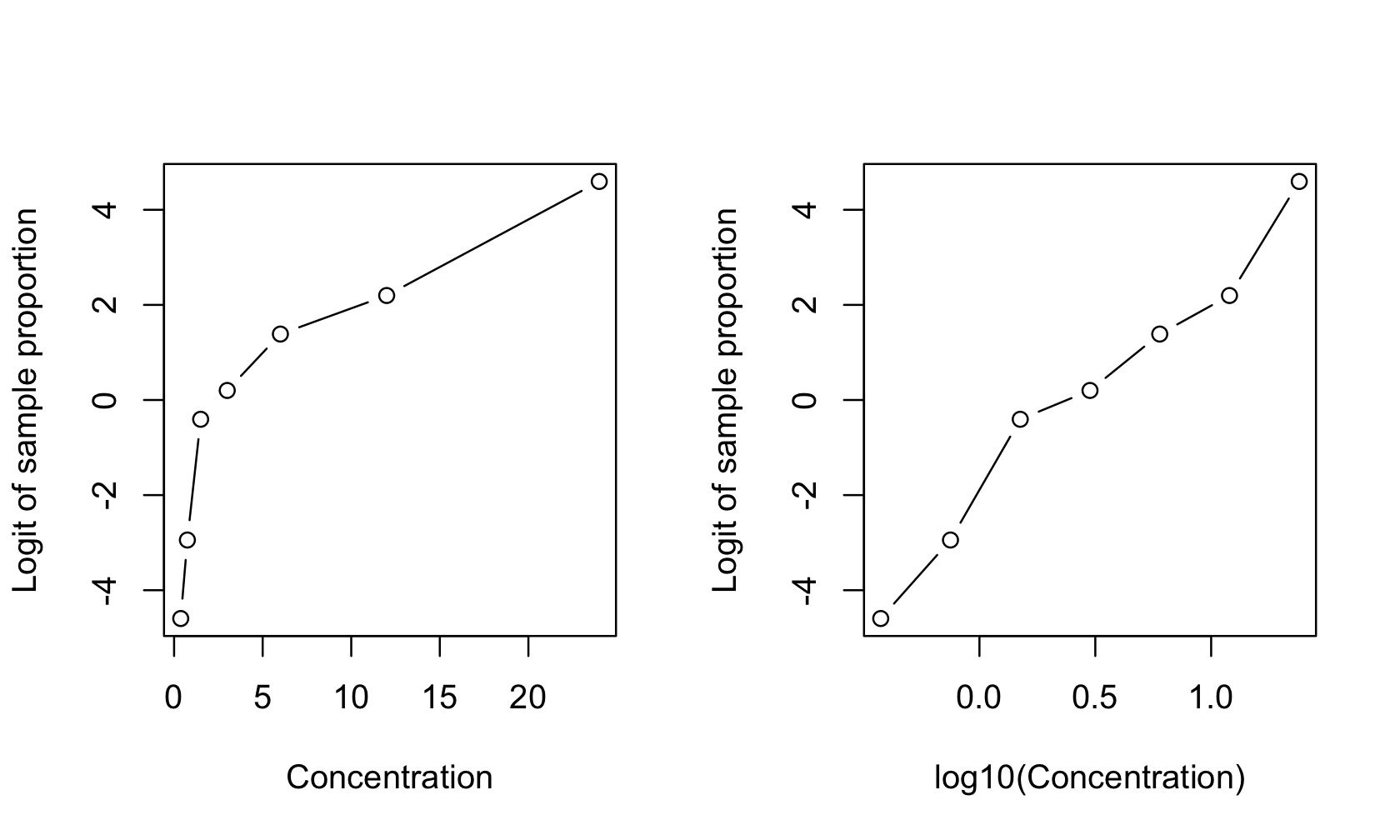
Example: Dose-response Study of Insect Mortality
Figure 23.8 shows logits of sample proportions in a dose-response study of insect larvae mortality as a function of the concentration of an insecticide. Suppose \(y_{i}\) denotes the number of larvae out of \(n_{i}\) that succumb to the insecticide at concentration \(x_{i}\). The right panel of the figure shows the logit of the sample proportion \(p_{i} = \frac{y_{i}}{n_{i}}\),
\[ \log\left\{ \frac{p_{i}}{1 - p_{i}} \right\} \]
as a function of the log insecticide concentration. A simple linear model seems appropriate,
\[ \log\left\{ \frac{\text{E}\lbrack p_{i}\rbrack}{1 - \text{E}\lbrack p_{i}\rbrack} \right\} = \beta_0 + \beta_1\log_{10}x_i \]
Note that the expected value \(\text{E}\left\lbrack p_{i} \right\rbrack\) is a probability. This model is a generalization of logistic regression for binary data (a 0/1 response) to binomial sample proportions. \(\text{E}\left\lbrack p_{i} \right\rbrack = \pi_{i}\) is the probability that an insect dies when \(\log_{10}x_{i}\) amount of insecticide is applied.
The investigators want to understand the relationship between larvae mortality and insecticide concentration. The parameter estimate for \(\beta_{1}\) is of interest, it describes the change in logits that corresponds to a unit-level change in the log concentration. A hypothesis test for \(\beta_{1}\) might compare the dose-response in this study with the known dose-response slope \(c\) of a standard insecticide. The null hypothesis of this test specifies that the insecticide is as effective as the standard:
\[ H_{0}:\beta_{1} = c \]
Another value of interest in dose-response studies is the concentration that achieves a specified effect. For example, the lethal dosage \(LD_{50}\) is the concentration that kills 50% of the subjects. Determining the \(LD_{50}\) value is known as an inverse prediction problem: rather than predicting \(\text{E}\lbrack Y\rbrack\) for a given value of \(X\), we are interested in finding the value \(X\) that corresponds to a given a value of \(\text{E}\lbrack Y\rbrack\).
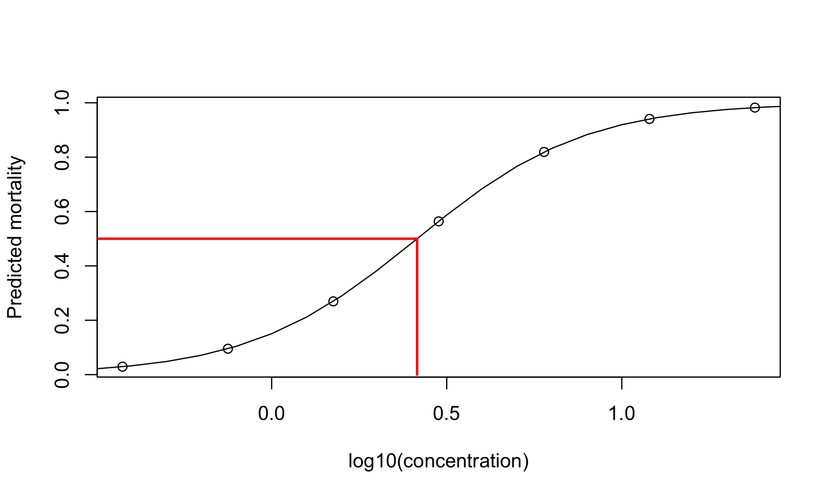
The \(LD_{50}\) value can be calculated from the model equation. More generally, we can find any value on the x-axis that corresponds to a particular mortality rate \(\alpha\) by solving the following equation for \(\alpha\):
\[ \text{logit}(\alpha) = \log\left\{ \frac{\alpha}{1 - \alpha} \right\} = \beta_0 + \beta_1\log_{10}x_\alpha \]
The solution is
\[ x_{\alpha} = 10^{\frac{\left( \text{logit}(\alpha) - \beta_{0} \right)}{\beta_{1}}} \]
For the special value \(\alpha = 0.5\), the \(LD_{50}\) results,
\[ LD_{50} = 10^{\frac{- \beta_{0}}{\beta_{1}}} \]
In addition to hypothesis testing about \(\beta_{1}\) and calculating the \(LD_{50}\), the investigators are also interested in predicting the mortality rate at concentrations not used in the study.
The inference in the study has explanatory (confirmatory) and predictive elements.
Many studies are not completely confirmatory or predictive, because models that are good at confirmatory inference are not necessarily good at predicting. Similarly, models that predict well are not necessarily good at testing hypotheses. Interpretability of the model parameters is important for confirmatory inference because hypotheses about the real world are cast as statements about the model parameters. Many disciplines place a premium on interpretability, e.g., biology, life sciences, economics, physical sciences, geo sciences, natural resources, financial services. Experiments designed to answer specific questions rely on analytic methods designed for confirmatory inference.
Interpretability of the model parameters might not be important for a predictive model. A biased estimator that reduces variability and leads to a lower mean squared prediction error (see Section 25.3) can be appealing in a predictive model but can be unacceptable in a project where confirmatory inference is the primary focus.
23.5 Interactions
Adding interactions between input features to a model can improve performance or can lead to overfitting. Interactions are built automatically into some statistical learning methods, for example, decision trees. In other cases you have to explicitly add them to the model.
As critically important as interactions are in modeling data, their concept is often poorly understood. Pitter patter—let’s get at ’er.
What is the difference between the following models \[ Y = \beta_0 + \beta_1 x_1 + \beta_2 x_2 + \epsilon \tag{23.1}\]
\[ Y = \beta_0 + \beta_1 x_1 + \beta_2 x_2 + \beta_3 x_1 x_2 + \epsilon \tag{23.2}\]
Both models depend on \(x_1\) and \(x_2\). In the first case the variables enter the model as main effects, that is, by themselves. Model Equation 23.2 also includes an interaction term, \(x_1 x_2\). You can think of this as a new feature, \(z=x_1 x_2\) and write the model as \(Y = \beta_0 + \beta_1 x_1 + \beta_2 x_2 + \beta_3 z + \epsilon\), but that obscures the fact that \(z\) is the product of two other input features. To be more precise, this is a two-way interaction term because it involves two input variables. A three-way interaction term would be \(x_1 x_2 x_3\).
Definition
In a model that consists of main effects only, each input variable
makes its contribution on the outcome given the presence of the other. To measure the change in the mean response when \(x_1\) changes by one unit it does not matter which value \(x_2\) takes on. In Equation 23.1, \(\beta_1\) measures the change in \(\text{E}[Y]\) when \(x_1\) increases by one unit.
Now consider the two-way interaction model Equation 23.2 and \(\beta_3\) is not zero. We can no longer state that \(\beta_1\) measures the effect on \(\text{E}[Y]\) when \(x_1\) is changed by one unit. The effect of changing \(x_1\) by one unit is now a function of \(x_2\). To see this, consider the mean of \(Y\) at two points, \(x_1\) and \(x_1+1\).
\[\begin{align*} \text{E}[Y | x_1] &= \beta_0 + \beta_1 x_1 + \beta_2 x_2 + \beta_3 x_1 x_2 \\ \text{E}[Y | x_1 + 1] &= \beta_0 + \beta_1 (x_1+1) + \beta_2 x_2 + \beta_3 (x_1+1)x_2 \end{align*}\]
The difference between the two is \[ \text{E}[Y | x_1 + 1] - \text{E}[Y | x_1] = \beta_1 + \beta_3 x_2 \]
The effect of \(x_1\) is now a function of \(x_2\). That is the very meaning of an interaction. The effect of one variable (or factor) depends on another variable (or factor) and vice versa. In the example, the effect of \(x_1\) is a linear regression in \(x_2\).
Definition: Interaction
Two variables \(X_1\) and \(X_2\) are said to interact if the effect of \(X_1\) depends on the values of \(X_2\), and vice versa. \(X_1\) and \(X_2\) can be continuous variables or qualitative factors. When both are factors, their interaction means that comparisons (contrasts) among the levels of one factor change with levels of the other factor.
For example, if \(A\) is a treatment factor with three levels (Placebo, Low Dose, High Dose), and \(B\) is a two-level gender factor (Male/Female), their interaction means that a comparison between low and high dose treatments yields different results for males and females. Expressed differently, a comparison of genders cannot be made without knowing what treatments were received. On the other hand, if the factors do not interact, then the difference between low dose and high dose response is the same for males and females.
This example shows how important it is to include interactions in models, if these are necessary. Omitting an interaction between variables can lead to bad conclusions. On the other hand, including all possible interactions is also not a good idea, it can lead to overfitting.
Global Interactions
The concept of interaction can be easily visualized for a model with a continuous and a two-level categorical input variable. Figure 23.10 displays on the left the situation where the variables do not interact and on the right the interaction case. With a two-level categorical factor, representing for example, a treatment and a placebo, the absence of interactions manifests itself in parallel lines. The effect of the treatment is the distance between the two lines and is the same for all values of \(x_1\). Similarly, the effect of \(x_1\), the slope of the line, is the same for both groups. In the presence of an interaction the slopes are not the same and the distance between the lines (the effect of \(x_2\)) depends on the value for \(x_1\).
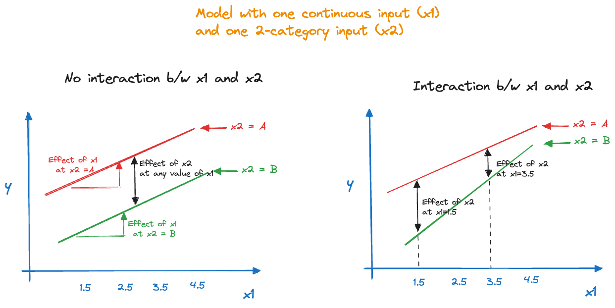
These interactions are also called global interactions, because they model joint behavior of two or more features over the entire range of the data. The term \(\beta_2 x_1 x_2\) does not depend on which values \(x_1\) or \(x_2\) take on, respectively. A local interaction model would capture the interactions differently for different segments of the data. For example, the following model captures local interactions by segmenting along \(I(x_2 \le c)\): \[ \text{E}[Y] = \beta_0 + \beta_1 x_1 + \beta_2 x_2 + \beta_3 x_1x_2\, I(x_2 \le c) + \beta_4 x_1 x_2 \, I(x_2 > c) \] If \(x_2 \le c\) the local interaction adds \(\beta_3x_1x_2\) to the mean and if \(x_2 > c\) the local interaction adds \(\beta_4 x_1 x_2\) to the mean. As you can see from this example, modeling interactions locally is possible in regression models, but it is tedious. If the threshold \(c\) is a parameter, the model becomes nonlinear. If the threshold is a constant, it needs to be determined based on exploratory data analysis and/or domain knowledge. Other learning methods incorporate local interactions more naturally, for example, decision trees (see below).
Tip
When building models with interactions, it is customary to include lower-order effects in the model if higher-order effects are significant. For example, if \(x_1 x_2\) is in the model one includes the main effects \(x_1\) and \(x_2\) regardless of their significance. Similarly, if a three-way interaction is significant one includes the two-way interactions and the main effects in the model. The argument for doing so is that in order for two things to interact they must be present—otherwise, what interacts?
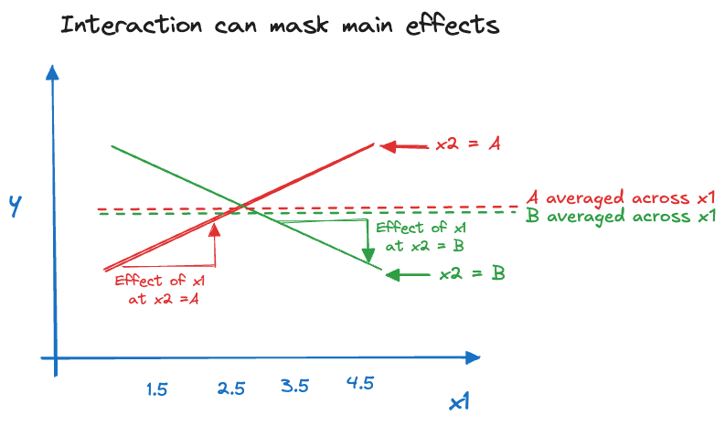
Figure 23.11 depicts the situation where the interaction between two inputs appears to remove the main effect. The crossing of the trends—due to a positive slope for group A and a negative slope for group B—leads to the averages of the two groups across the values of \(x\) (the main group effects) to be very similar. We say in this case that the interaction between \(x_1\) and \(x_2\) masks the main effect of \(x_2\). You recognize this phenomenon when interaction terms are statistically significant but one or more main effects involved in the interactions are not. If we keep the interaction in the model, we would also keep their main effects.
It is tempting to add interactions between all features and higher-order interactions as well. The argument is that one does not miss any potentially important dependence between the variables. The counter argument is that including unimportant features in a model is not without cost. Variables that do not carry information toward the target—given all other variables in the model—reduce the overall loss function but they can lead to overfitting and make the model perform worse overall. The following example demonstrates this for a simple data set. By increasing the number and order of interaction terms the \(R^2\) statistic increases. The PRESS statistic measures the ability of a model to predict a new observation that was not used in training. Initially, adding more terms improves the PRESS statistic (its value decreases). At some point the model is overfit and adding more interaction terms reduces the predictive power of the model. (More on PRESS and mean squared error-based measures of model performance in Section 25.3.)
Example: Auto Data
The Auto data in the ISLR2 package in R provides gas mileage, horsepower, displacement, and other characteristics for 396 automobiles. We are considering a series of increasingly complex linear models, culminating in a model with four main effects and four-way interactions.
The first four models add inputs and also two-way interactions of all inputs in the model. The formula expression y ~ (x1 + x2 + x3)^2 is a shorthand for including the main effects and two-way interactions of the three inputs. R displays the interaction terms as x1:x2, x1:x3, and x2:x3 in the output.
Model 1 is a simple linear regression model \[
\text{E}[\text{mpg}] = \beta_0 + \beta_1 \,\text{cylinders}
\] Model 2 adds displacement and the two-way interaction with cylinders: \[
\text{E}[\text{mpg}] = \beta_0 + \beta_1 \,\text{cylinders} + \beta_2 \,\text{displacement}
+ \beta_3 \,\text{cylinders}\times\text{displacement}
\] Model 3 adds the horsepower feature and includes three two-way interactions: cylinders x displacement, cylinders x horsepower, and displacement x horsepower.
Models 5 and 6 then add up to three-way and four-way interactions, respectively. For each model we calculate the number of non-zero coefficients (the rank of \(\textbf{X}\)), SSE, \(R^2\) and the PRESS statistic.
library(ISLR2)
data(Auto)

calcPress <- function(linModel) {
    leverage <- hatvalues(linModel)
    r <- linModel$residuals
    Press_res <- r/(1-leverage)
    Press <- sum(Press_res^2)
    return(list("ncoef"=linModel$rank,
                "R2"   =summary(linModel)$r.squared,
                "SSE"  =sum(r^2),
                "PRESS"=Press))
}

l1 <- lm(mpg ~ cylinders, data=Auto)
l2 <- lm(mpg ~ (cylinders + displacement)^2, data=Auto )
l3 <- lm(mpg ~ (cylinders + displacement + horsepower)^2, data=Auto )
l4 <- lm(mpg ~ (cylinders + displacement + horsepower + weight)^2, data=Auto )
l5 <- lm(mpg ~ (cylinders + displacement + horsepower + weight)^3, data=Auto )
l6 <- lm(mpg ~ (cylinders + displacement + horsepower + weight)^4, data=Auto )

df <- rbind(as.data.frame(calcPress(l1)),
            as.data.frame(calcPress(l2)),
            as.data.frame(calcPress(l3)),
            as.data.frame(calcPress(l4)),
            as.data.frame(calcPress(l5)),
            as.data.frame(calcPress(l6))
      )
knitr::kable(df,format="simple")| ncoef | R2 | SSE | PRESS |
|---|---|---|---|
| 2 | 0.6046890 | 9415.910 | 9505.534 |
| 4 | 0.6769104 | 7695.670 | 7846.982 |
| 7 | 0.7497691 | 5960.247 | 6197.767 |
| 11 | 0.7607536 | 5698.608 | 6089.687 |
| 15 | 0.7752334 | 5353.714 | 5818.953 |
| 16 | 0.7752893 | 5352.382 | 5861.117 |
The model complexity increases from the first to the sixth model; the models have more parameters and more intricate interaction terms. The SSE values decrease as terms are added to the model, and \(R^2\) increases accordingly. The PRESS statistic is always larger than the SSE, which makes sense because it is based on squaring the Press residuals \((y_i - \widehat{y}_i)/(1-h_{ii})\) which are larger than the ordinary residuals \(y_i - \widehat{y}_i\).
From the fifth to the sixth model only one additional parameter is added to the model, the four-way interaction of all inputs. \(R^2\) barely increases but the PRESS statistic increases compared to the model with only three-way interaction. Interestingly, none of the effects in the four-way model are significant given the presence of other terms in the model.
summary(l6)
Call:
lm(formula = mpg ~ (cylinders + displacement + horsepower + weight)^4,
    data = Auto)

Residuals:
     Min       1Q   Median       3Q      Max
-12.0497  -1.9574  -0.2334   1.8091  18.8569

Coefficients:
                                           Estimate Std. Error t value Pr(>|t|)
(Intercept)                               6.104e+01  7.744e+01   0.788    0.431
cylinders                                -4.974e+00  1.465e+01  -0.339    0.734
displacement                             -4.338e-01  5.655e-01  -0.767    0.444
horsepower                               -6.459e-01  7.861e-01  -0.822    0.412
weight                                    2.735e-02  2.623e-02   1.042    0.298
cylinders:displacement                    4.737e-02  7.861e-02   0.603    0.547
cylinders:horsepower                      1.069e-01  1.324e-01   0.808    0.420
cylinders:weight                         -2.757e-03  4.565e-03  -0.604    0.546
displacement:horsepower                   8.090e-03  6.253e-03   1.294    0.197
displacement:weight                      -7.045e-05  1.775e-04  -0.397    0.692
horsepower:weight                        -2.047e-04  2.689e-04  -0.761    0.447
cylinders:displacement:horsepower        -1.041e-03  8.238e-04  -1.263    0.207
cylinders:displacement:weight             8.719e-06  2.422e-05   0.360    0.719
cylinders:horsepower:weight               1.351e-05  4.130e-05   0.327    0.744
displacement:horsepower:weight           -4.645e-07  1.920e-06  -0.242    0.809
cylinders:displacement:horsepower:weight  7.702e-08  2.517e-07   0.306    0.760

Residual standard error: 3.773 on 376 degrees of freedom
Multiple R-squared:  0.7753,    Adjusted R-squared:  0.7663
F-statistic: 86.48 on 15 and 376 DF,  p-value: < 2.2e-16
The first four models add inputs and also two-way interactions of all inputs in the model. The code uses patsy’s dmatrices function to build model expressions similar to the formula expression in R.
Model 1 is a simple linear regression model \[
\text{E}[\text{mpg}] = \beta_0 + \beta_1 \,\text{cylinders}
\] Model 2 adds displacement and the two-way interaction with cylinders: \[
\text{E}[\text{mpg}] = \beta_0 + \beta_1 \,\text{cylinders} + \beta_2 \,\text{displacement}
+ \beta_3 \,\text{cylinders}\times\text{displacement}
\] Model 3 adds the horsepower feature and includes three two-way interactions: cylinders x displacement, cylinders x horsepower, and displacement x horsepower.
Models 5 and 6 then add up to three-way and four-way interactions, respectively. For each model we calculate the number of non-zero coefficients (the rank of \(\bX\)), SSE, \(R^2\) and the PRESS statistic.
import statsmodels.api as sm
import pandas as pd
import numpy as np
from patsy import dmatrices
from tabulate import tabulate
import duckdb

con = duckdb.connect(database="../ads.ddb", read_only=True)
Auto_data = con.sql("SELECT * FROM auto").df().dropna()
con.close()

# Define function to calculate PRESS and other statistics
def calc_press(model):
    leverage = model.get_influence().hat_matrix_diag
    r = model.resid
    press_res = r / (1 - leverage)
    press = np.sum(press_res**2)

    return {
        "ncoef": model.df_model + 1,  # +1 for intercept
        "R2": model.rsquared,
        "SSE": np.sum(r**2),
        "PRESS": press
    }

formula1 = "mpg ~ cylinders"
y, X = dmatrices(formula1, data=Auto_data, return_type='dataframe')
l1 = sm.OLS(y, X).fit()

formula2 = "mpg ~ (cylinders + displacement)**2"
y, X = dmatrices(formula2, data=Auto_data, return_type='dataframe')
l2 = sm.OLS(y, X).fit()

formula3 = "mpg ~ (cylinders + displacement + horsepower)**2"
y, X = dmatrices(formula3, data=Auto_data, return_type='dataframe')
l3 = sm.OLS(y, X).fit()

formula4 = "mpg ~ (cylinders + displacement + horsepower + weight)**2"
y, X = dmatrices(formula4, data=Auto_data, return_type='dataframe')
l4 = sm.OLS(y, X).fit()

formula5 = "mpg ~ (cylinders + displacement + horsepower + weight)**3"
y, X = dmatrices(formula5, data=Auto_data, return_type='dataframe')
l5 = sm.OLS(y, X).fit()

formula6 = "mpg ~ (cylinders + displacement + horsepower + weight)**4"
y, X = dmatrices(formula6, data=Auto_data, return_type='dataframe')
l6 = sm.OLS(y, X).fit()

df = pd.DataFrame([
    calc_press(l1),
    calc_press(l2),
    calc_press(l3),
    calc_press(l4),
    calc_press(l5),
    calc_press(l6)
])

print(tabulate(df, headers='keys', tablefmt='simple'))
ncoef R2 SSE PRESS
-- ------- -------- ------- -------
0 2 0.604689 9415.91 9505.53
1 4 0.67691 7695.67 7846.98
2 7 0.749769 5960.25 6197.77
3 11 0.760754 5698.61 6089.69
4 15 0.775233 5353.71 5818.95
5 16 0.775289 5352.38 5861.12print(l6.summary()) OLS Regression Results
==============================================================================
Dep. Variable: mpg R-squared: 0.775
Model: OLS Adj. R-squared: 0.766
Method: Least Squares F-statistic: 86.48
Date: Wed, 22 Oct 2025 Prob (F-statistic): 9.05e-112
Time: 10:15:17 Log-Likelihood: -1068.6
No. Observations: 392 AIC: 2169.
Df Residuals: 376 BIC: 2233.
Df Model: 15
Covariance Type: nonrobust
============================================================================================================
coef std err t P>|t| [0.025 0.975]
------------------------------------------------------------------------------------------------------------
Intercept 61.0371 77.437 0.788 0.431 -91.227 213.301
cylinders -4.9738 14.653 -0.339 0.734 -33.786 23.839
displacement -0.4338 0.566 -0.767 0.444 -1.546 0.678
horsepower -0.6459 0.786 -0.822 0.412 -2.192 0.900
weight 0.0273 0.026 1.042 0.298 -0.024 0.079
cylinders:displacement 0.0474 0.079 0.603 0.547 -0.107 0.202
cylinders:horsepower 0.1069 0.132 0.808 0.420 -0.153 0.367
cylinders:weight -0.0028 0.005 -0.604 0.546 -0.012 0.006
displacement:horsepower 0.0081 0.006 1.294 0.197 -0.004 0.020
displacement:weight -7.045e-05 0.000 -0.397 0.692 -0.000 0.000
horsepower:weight -0.0002 0.000 -0.761 0.447 -0.001 0.000
cylinders:displacement:horsepower -0.0010 0.001 -1.263 0.207 -0.003 0.001
cylinders:displacement:weight 8.719e-06 2.42e-05 0.360 0.719 -3.89e-05 5.63e-05
cylinders:horsepower:weight 1.351e-05 4.13e-05 0.327 0.744 -6.77e-05 9.47e-05
displacement:horsepower:weight -4.645e-07 1.92e-06 -0.242 0.809 -4.24e-06 3.31e-06
cylinders:displacement:horsepower:weight 7.702e-08 2.52e-07 0.306 0.760 -4.18e-07 5.72e-07
==============================================================================
Omnibus: 51.766 Durbin-Watson: 1.035
Prob(Omnibus): 0.000 Jarque-Bera (JB): 136.295
Skew: 0.636 Prob(JB): 2.53e-30
Kurtosis: 5.594 Cond. No. 4.33e+11
==============================================================================
Notes:
[1] Standard Errors assume that the covariance matrix of the errors is correctly specified.
[2] The condition number is large, 4.33e+11. This might indicate that there are
strong multicollinearity or other numerical problems.Local Interactions in Decision Trees
In the regression model we have to explicitly incorporate interactions. This raises the question which variables interact and the appropriate highest order of the interaction terms. Some form of feature selection method needs to be applied to make sure the model does not get out of hand and overfit.
Other statistical learning techniques incorporate interaction effects more naturally. A great example are decision trees. Their intrinsic interpretability is an often-cited advantage. Another benefit of decision trees is the modeling of interactions and nonlinearity. In addition, decision trees model local interactions, rather than the global interactions in regression models.
This is best explained with an example. Figure 23.12 displays a simple decision tree with three terminal nodes. The fist split at the trunk of the tree is on the Age variable. Observations with Age <= 20 are not split further. On the right branch the tree is split once more by the Amount variable.
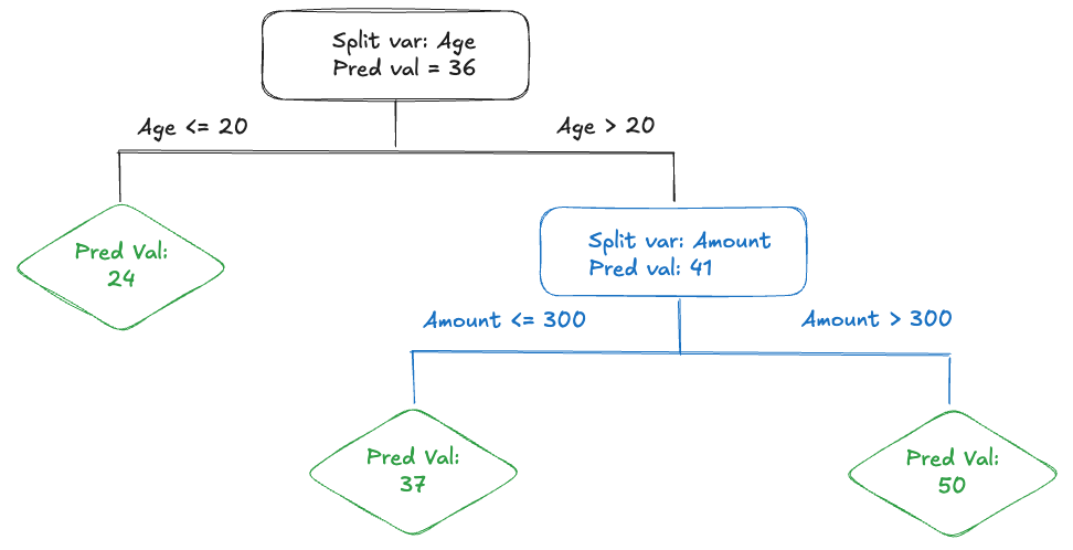
How do the splits relate to the interaction of features? Recall the definition of the interaction between \(x_1\) and \(x_2\): The effect of \(x_1\) (\(x_2\)) depends on the value of \(x_2\) (\(x_1\)). In the decision tree a conclusion about the effect of Age on the predicted value cannot be made without knowing the value of the Amount variable. Similarly, the effect of Amount on the predicted value cannot be known without identifying the side of the tree you are in, that is, which Age category you are in.
Decision trees naturally model interactions and the order of the interaction is given by the number of features involved between the trunk and a terminal node. Since variables can be re-used at lower split points, it is not correct to say that the depth of the tree is identical to the order of the interaction. You have to count the number of unique variables in a branch.
Furthermore, the interactions modeled by the decision tree are local. To see this, we can express the predicted values in the terminal nodes through model formulas. Specifically,
\[ \begin{align*} \text{PredVal}_1 &= 24\times I\left(\text{Age} \le 20\right) \\ \text{PredVal}_2 &= 37\times I\left(\text{Age} > 20 \right) \times I\left(\text{Amount} \le 300 \right) \\ \text{PredVal}_3 &= 50\times I\left(\text{Age} > 20 \right) \times I\left(\text{Amount} > 300 \right) \end{align*} \]
The tree captures interactions differently for ranges of the input features.