Data quality is a massive topic and hugely important in data science. You know the adage “garbage in, garbage out”. It is part of data engineering and the not-so-sexy part of working with data. How we would love to start our data science projects from the best possible data of the highest data quality. Unfortunately, that is not how many projects work.
If you work in an organization with a dedicated data engineering team, then many of the tasks involved in assessing and increasing data quality fall on that team. As a data scientist, you still need to be keenly aware of the quality issues around data, how to identify them, and how to fix them. If you operate in a smaller organization, data quality assessments and corrections might fall on you.
Preprocessing
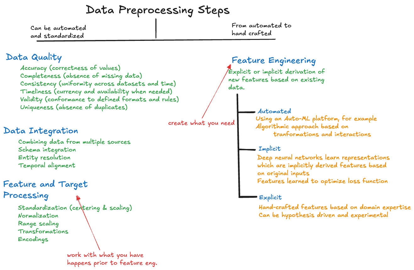
Data quality is just one of many data preprocessing steps, each has several dimensions (Figure 28.1). Feature/target processing and feature engineering are definitely activities where the data scientist is involved.
Figure 16.1: Data preprocessing steps. Click to enlarge.
In this chapter we deal with data issues in a single data source. A separate set of issues arises when data are combined across different sources. That is the topic of Chapter 19. For example, two data sets contain time-based information and their timestamps are complete, without missing values or duplicates. The quality of the timestamp information is high. When the two data sets are merged it turns out that the information in one data set is based on ISO 8601 timestamps and the other is based on Unix time. This needs to be resolved before the data sets can be merged (integrated).
Data Quality Dimensions
The quality of a data source is assessed across a number of dimensions:
Accuracy
How closely data matches real-world values
Accuracy measures how well data reflects the true state of the real world it represents. When a customer’s age is recorded as 150 years old or their annual income is listed as negative, these values fail the accuracy test because they do not correspond to reality. Accuracy issues often stem from measurement errors, data entry mistakes, or system integration problems that introduce distortions between the actual phenomenon and its recorded representation.
Completeness
Extent to which data are present and not missing
Assessment: Percentage of filled vs. empty fields
Issues: Null values, missing values, partial records
Completeness refers to the extent to which all required data elements are present and populated in the data. Missing values, empty fields, and null entries are completeness problems that can significantly impact analysis outcomes.
Consistency
Data uniformity across systems and time
Issues: Different formats, conflicting values, timing differences
Consistency ensures that data follow uniform standards and formats throughout the data set and across different systems. When the same information is represented differently, for example, recording states as “CA,” “California,” and “ca” within the same database, it creates consistency problems that complicate analysis.
Consistency also extends to logical relationships. If someone’s age is 25 years based on a birth date field but the age column indicates they are 45 years old, then the data are not internally consistent.
Timeliness
How current and up-to-date the data are
Assessment: Data freshness, update frequency
Issues: Batch delays, system latency, manual processes, mix of current and outdated records
Timeliness evaluates whether data are current, up-to-date, and available when needed for decision-making purposes. Data that are accurate when first collected can become stale or irrelevant as time passes. Customer contact details, product information, or inventory levels can change quickly.
Validity
Data conformance to defined formats and rules
Assessment: Format validation, business rule compliance
Issues: Invalid formats, constraint violations, range errors
Validity determines whether data conforms to defined formats, rules, and acceptable value ranges within its intended domain. A phone number containing letters, an email address missing the “@” symbol, or a credit score outside the 300-850 range represent validity violations. Valid data adheres to business rules, technical constraints, and logical boundaries that define what constitutes acceptable values for each data element.
Databases allow you to specify constraints when defining columns of a table. These can ensure that invalid entries do not make it into the data.
Uniqueness
Absence of duplicate records or values
Assessment: Duplicate detection algorithms
Issues: Multiple identifiers, data entry errors, system integration, duplicate rows
Uniqueness ensures that each real-world entity is represented only once within the data, preventing duplicate records that can skew analysis and waste resources. When the same customer appears multiple times with slight variations in their information, it creates uniqueness problems that inflate counts, distort statistical measures, and complicate customer relationship management. Effective uniqueness management requires sophisticated matching algorithms that can identify duplicates despite minor differences in how the same entity might be recorded.
16.2 Data Profiling
Data profiling is a diagnostic tool for data quality and reveals data quality issues. Profiling a data set means to systematically examine its structure, content, and relationships to uncover quality problems like missing values, outliers, inconsistent formats, duplicate records, or constraint violations.
Data profiling is one of the first activities when you encounter a new data set. (Borne 2021) refers to it as “having that first date with your data.” It is how you kick-start the exploratory data analysis (EDA).
Think of data profiling as the medical examination phase of data quality management. Just as a doctor runs tests to diagnose health issues before prescribing treatment, data profiling identifies quality problems before you can address them. The result of data profiling—statistical summaries, distribution analyses, pattern detection, and anomaly identification—feed into data quality improvement decisions.
While in theory the profiling results inform the data quality strategy, in practice the lines blur and profiling is bundled with initial data quality fixes. When you notice that a column has inconsistent date formats, you might fix them before moving on to the next column.
Data profiling without subsequent quality improvement is incomplete, while quality improvement without proper profiling is often misguided. The two activities are complementary phases of ensuring your data meets the standards required for reliable analysis.
The First Date with your Data
We are not looking to derive new insights from the data or to build amazing machine learning models during profiling; we want to create a high-level report of the data content and condition. We want to know what we are dealing with. Common questions and issues addressed during profiling are
Which variables (attributes) are in the data?
How many rows and columns are there?
Which variables are quantitative (represent numbers), and which variables are qualitative (represent class memberships)
Are qualitative variables coded as strings, objects, numbers?
Are there complex data types such as JSON documents, images, audio, video encoded in the data?
What are the ranges (min, max) of the variables. Are these reasonable or do they suggest outliers or measurement errors?
What is the distribution of quantitative variables?
What is the mean, median, and standard deviation of quantitative variables?
What are the unique values of qualitative variables?
Do coded fields such as ZIP codes, account numbers, email addresses, state codes have the correct format?
Are there attributes that have only a single value?
Are there duplicate entries?
Are there missing values in one or more variables?
What are the strengths and direction of pairwise associations between the variables?
Are some attributes perfectly correlated, for example, birthdate and age or temperatures in degree Celsius and degree Fahrenheit.
California Housing Prices
In this subsection we consider a data set on housing prices in California, based on the 1990 census and available on Kaggle. The data contain information about geographic location, housing, and population within blocks. California has over 8,000 census tracts and a tract can have multiple block groups. There are over 20,000 census block groups and over 700,000 census blocks in California.
The variables in the data are:
Variables in the California Housing Prices data set.
Variable
Description
longitude
A measure of how far west a house is; a higher value is farther west
latitude
A measure of how far north a house is; a higher value is farther north
housing_median_age
Median age of a house within a block; a lower number is a newer building
total_rooms
Total number of rooms within a block
total_bedrooms
Total number of bedrooms within a block
population
Total number of people residing within a block
households
Total number of households, a group of people residing within a home unit, for a block
median_income
Median income for households within a block of houses (measured in tens of thousands of US Dollars)
median_house_value
Median house value for households within a block (measured in US Dollars)
ocean_proximity
Location of house with respect to ocean/sea
The variable description is important metadata to understand the data. A variable such as totalRooms could be understood as the number of rooms in a building and the medianHouseValue could then mean the median of the houses that have that number of rooms. However, since the data are not for individual houses but blocks, totalRooms represents the sum of all the rooms in all the houses in that block.
We start data profiling a pandas DataFrame of the data with getting basic info and a listing of the first few observations.
import pandas as pdimport duckdbcon = duckdb.connect(database="../ads.ddb", read_only=True)CA_houses = con.sql("SELECT * FROM california").df()con.close()CA_houses.info()
   longitude  latitude  ...  median_house_value  ocean_proximity
0    -122.23     37.88  ...            452600.0         NEAR BAY
1    -122.22     37.86  ...            358500.0         NEAR BAY
2    -122.24     37.85  ...            352100.0         NEAR BAY
3    -122.25     37.85  ...            341300.0         NEAR BAY
4    -122.25     37.85  ...            342200.0         NEAR BAY

[5 rows x 10 columns]
We can immediately answer several questions about the data:
There are 20,640 rows and 10 columns
Except for ocean_proximity, which is of object type (string), all other variables are stored as 64-bit floats. Variables total_rooms, total_bedrooms, population, and households are naturally integers; since they appeared in the CSV file with a decimal point, they were assigned a floating point data type.
Only the total_bedrooms variable has missing values, 20,640 – 20,433 = 207 values for this variable are unobserved. This shows a high level of completeness of the data set. (More on missing values in the next section).
The listing of the first five observations confirms that variables are counts or sums at the block-level, rather than data for individual houses.
The latitude and longitude values differ in the second decimal place, suggesting that blocks (=rows of the data set) have unique geographic location, but we cannot be sure.
The ocean_proximity entries are in all caps. We want to see the other values in that column to make sure the entries are consistent. Knowing the format of strings is important for filtering (selecting) or grouping observations.
The next step is to use pandas describe() function to compute basic summaries of the variables.
For each of the numeric variables, describe() computes the number of non-missing values (count), the sample mean (mean), the sample standard deviation (std), the minimum (min), maximum (max) and three quartiles (25%, 50%, 75% percentiles).
The results confirm that all variables have complete data (no missing values) except for total_bedrooms. The min and max values are useful to see the range (range = max – min) for the variables and to spot outliers and unusual values. It is suspicious that there is one or more blocks with a single household. This is not necessarily the same record that has 2 total_rooms and a population of 3.
CA_houses[CA_houses["households"] ==1]
       longitude  latitude  ...  median_house_value  ocean_proximity
16171     -122.5     37.79  ...            500001.0         NEAR BAY

[1 rows x 10 columns]
This is indeed a suspicious record. There is a single household in the block, but thirteen people are living in the block in a house with eight rooms and one bedroom. An unusual configuration that should be examined for possible data entry errors.
Profiling Tools
You can accelerate the data profiling task by using packages such as ydata_profiling (f.k.a. pandas_profiling), lux, or sweetviz. Sweetviz, for example, generates detailed interactive visualizations in a web browser or a notebook that help to address some of the profiling questions we raised at the beginning of the section.
To create a profile report for the housing prices data with sweetviz, use the following:
import sweetviz as svmy_report = sv.analyze(CA_houses)
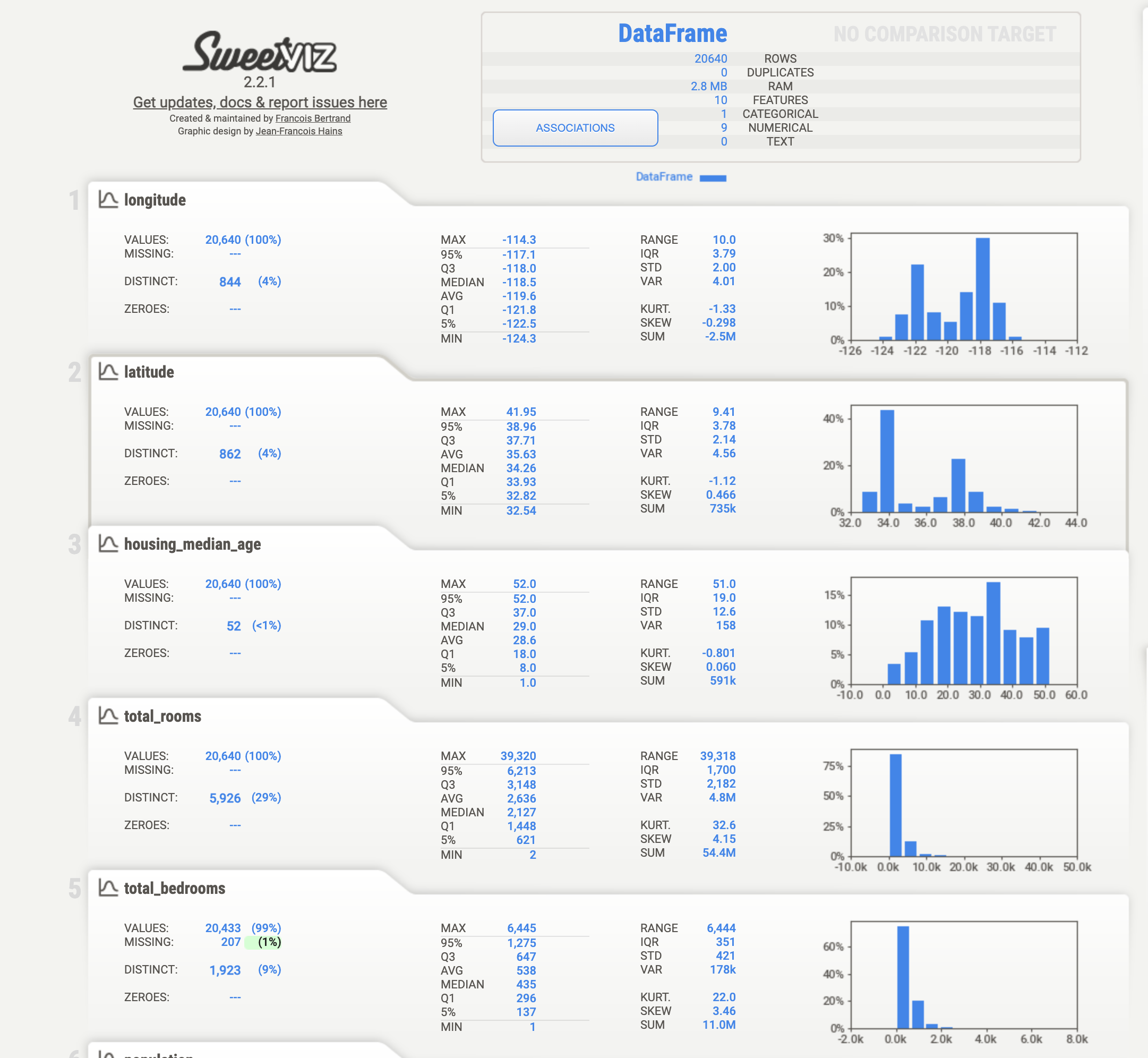
Figure 16.2 displays the main screen of the visualization. You can access the entire interactive html report here. For each numeric variable sweetviz reports the number of observed and missing values, the number of distinct values, and a series of summary statistics similar to the output from describe(). A histogram is also produced that gives an idea of the distribution of the variable in the data set. For example, housing_median_age has a fairly symmetric distribution, whereas total_rooms and total_bedrooms are highly concentrated despite a wide range.
Figure 16.2: Sweetviz visualization for California Housing Prices. Main screen, some numeric variables.
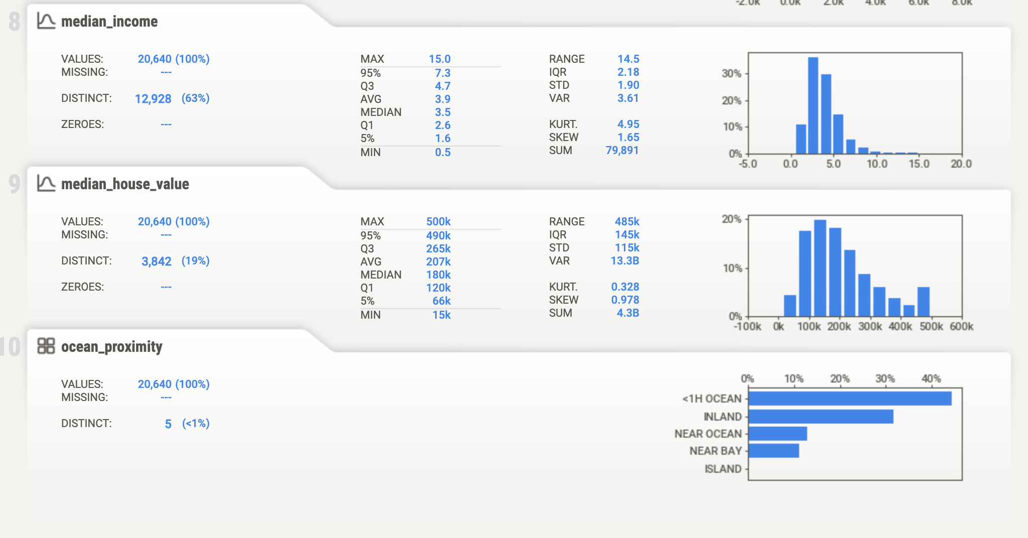
Figure 16.3 shows the bottom of the main screen that displays information on the ocean_proximity variable. We now see that there are five unique values for the variable with the majority in the category <1H OCEAN.
Figure 16.3: Profiling information for qualitative variable ocean_proximity.
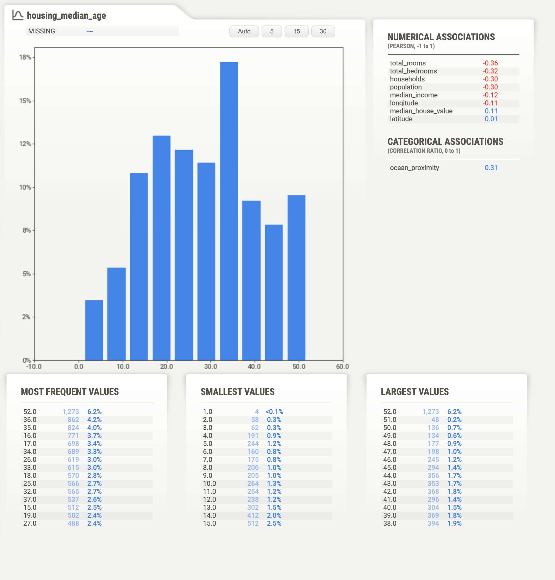
Clicking on any variable brings up more details. For housing_median_age that detail is shown in Figure 16.4. It includes a detailed histogram of the distribution, largest, smallest, and most frequent values.
Figure 16.4: Sweetviz detail for the variable housing_median_age.
The graphics are interactive, the number of histogram columns can be changed to the desired resolution.
Sweetviz displays pairwise associations between variables. You can see those for housing_median_age in Figure 16.4 or for all pairs of variables by clicking on Associations (Figure 16.5).
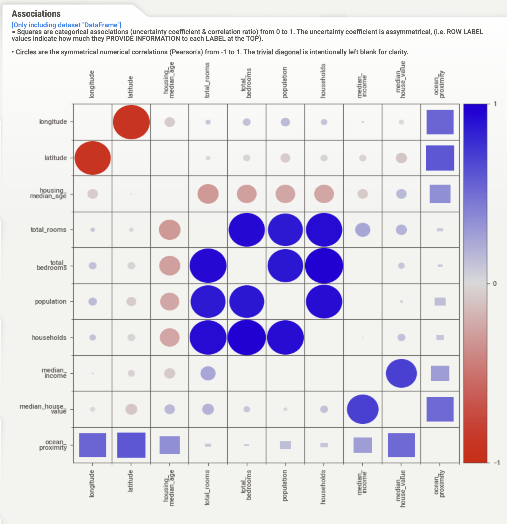
Figure 16.5: Sweetviz visualization of pairwise associations in California Housing Prices data.
Associations are calculated and displayed differently depending on whether the variables in a pair are quantitative or not. For pairs of quantitative variables, sweetviz computes the Pearson correlation coefficient. It ranges from –1 to +1; a coefficient of 0 indicates no (linear) relationship between the two variables, they are uncorrelated. A coefficient of +1 indicates a perfect positive correlation, knowing one variable allows you to perfectly predict the other variable. Similarly, a Pearson coefficient of –1 means that the variables are perfectly correlated and one variable decreases as the other increases.
Strong positive correlations are present between households and the variables total_rooms, total_bedrooms, and population. That is expected as these variables are accumulated across all households in a block. There is a moderate positive association between median income and median house value. More expensive houses are associated with higher incomes—not surprising. A strong negative correlation exists between longitude and latitude, a consequence of the geography of California: as you move further west (east) the state reaches further south (north).
Associations between quantitative and qualitative variables are calculated as the correlation ratio that ranges from 0 to 1 and displayed as squares in the Associations matrix. The correlation ratio is based on means within the categories of the qualitative variables. A ratio of 0 means that the means of the quantitative variable are identical for all categories. Since the data contains only one qualitative variable, ocean_proximity, squares appear only in the last row and column of the Associations matrix.
If the data contains an obvious target variable for modeling, you can indicate that when creating the profiling report. Sweetviz then adds information on that variable to the visualizations. Suppose that we are interested in modeling the median house value as a function of other attributes. The following statement requests a report with median_house_value as the target.
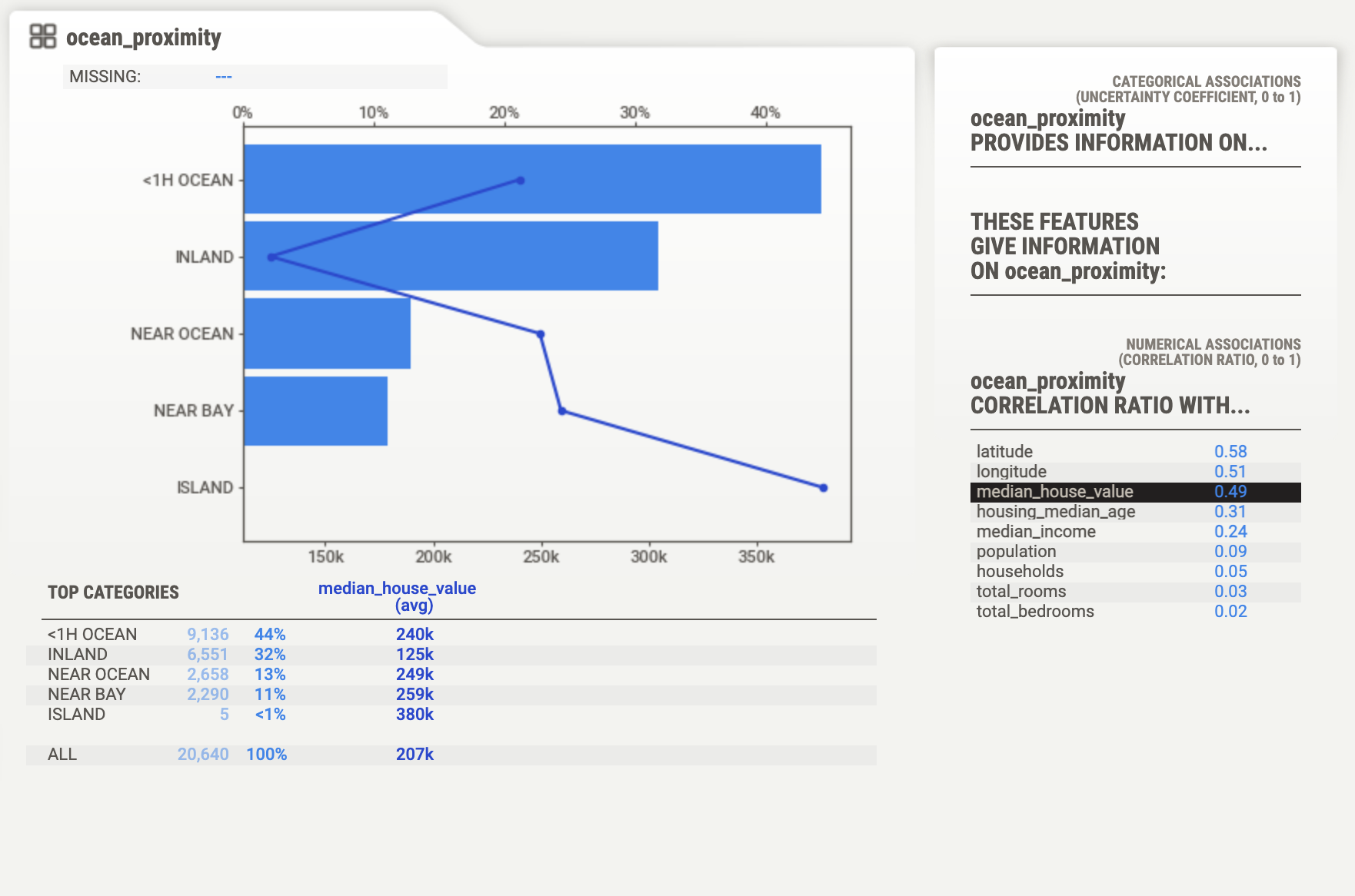
Figure 16.6 shows the detail on ocean_proximity from this analysis; the complete report is here. The average of the block’s median housing values in the five groups of ocean proximity are shown on top of the histogram. The highest average median house value is found on the island, the lowest average in the inland category.
Figure 16.6: Profiling details for ocean_proximity with target median_house_value.
16.3 Exercise: Customer Data Quality
The following code creates a data frame of 1,004 customer records with 15 attributes from the customer_quality table in the ads.ddb database. The data types vary from integers to strings (object type), floats, and datetime values. The column names are self explanatory.
import duckdbimport pandas as pdpd.set_option('display.max_columns', None)con = duckdb.connect(database="../ads.ddb", read_only=True)cust_info = con.sql("SELECT * FROM customer_quality;").df()con.close()print("Dataset created successfully!")
Based on the first five observations, a number of data quality issues are apparent: invalid formats (email), varying formats (phone), invalid values (age), outliers (annual_income), missing values (several), different spellings and abbreviations (state, country), and so on.
The next statements create the profile report, which can be seen here.
When an observation does not have a value assigned to it, we say that the value is missing. This is a fact of life in data analytics; whenever you work with a set of data you should expect values to be missing.
Definition: Missing Value
A missing value is an observation that has no value assigned to it.
Missingness is obvious when you see incomplete columns in the data. The problem can be inconspicuous when entire records are absent from the data. A survey that fails to include a key demographic misses the records of those who should have been sampled in the survey.
You should check the software packages used for data analysis on how they handle missing values—by default and how the behavior can be affected through options. In many cases the default behavior is casewise deletion, also known as complete-case analysis: any record that has a missing value in one or more of the analysis variables is excluded from the analysis. Pairwise deletion removes only those records that have missing values for a specific analysis. To see the difference, consider the data in Table 16.1 and suppose you want to compute the matrix of correlations among the variables.
Table 16.1: Three variables with different missing value patterns.
\(X_1\)
\(X_2\)
\(X_3\)
1.0
3.0
.
2.9
.
3.4
3.8
.
8.2
0.5
3.7
.
A complete-case analysis of \(X_1\), \(X_2\), and \(X_3\) would result in a data frame without observations since each row of the table has a missing value in one column. Pairwise deletion, on the other hand, computes the correlation between \(X_1\) and \(X_2\) based on the first and last observation, the correlation between \(X_1\) and \(X_3\) based on the second and third observation and fails to produce a correlation between \(X_2\) and \(X_3\).
What are some possible causes for missing values:
Members of the target population not included in sample (missing records)
Data entry errors
Variable transformations that lead to invalid values: division by zero, logarithm of zeros or negative values
Measurement equipment malfunction
Measurement equipment limits exceeded
Attrition (drop-out) of subject in longitudinal studies (death, moving, refusal, changes in medical condition, …)
Non-response of subjects in surveys
Variables not measured
Unobservable factor combinations. The data set of your Netflix movie ratings is extremely sparse, unless you “finished Netflix” and rated all movies
Regulatory requirements force removal of sensitive information
Data transformations can introduce missing values into data sets when mathematical operations are not valid. To accommodate nonlinear relationships between target and input variables, transformations of inputs such as ratios, square roots, and logarithms are common. These transformations are sometimes applied to change the distribution of data, for example, to create more symmetry by taking logarithms of right-skewed data (Figure 16.7).
Figure 16.7: Distribution of home values and logarithm of home values in Albemarle County, VA. The log-transformed data is more symmetric distributed. Since all home values are positive, the transformation does not create missing values.
In the home values example it is reasonable to proceed with an analysis that assumes the log(value) is Gaussian distributed. But suppose you are log-transforming another highly skewed variable, the amount of individual’s annual medical out-of-pocket expenses. Most people have a moderate amount of out-of-pocket expenses, a smaller percentage have very high annual expenses. However, many will have no out-of-pocket expenses at all. Taking the logarithm will invalidate the records of those individuals. To get around the numerical issue of taking logarithms of zeros, transformations are sometimes adjusted to use log(expenses+1) instead of log(expenses). This avoids missing values but fudges the data by pretending that everyone has at least some medical expenses.
Software packages are quick to throw out records with missing values in the analysis variables. Removing missing values from the analysis is appropriate only when the reason for the missingness is not related to any other information in the study. For example, if you study the weight of animals and a measurement is not included because the scales randomly break, then the analysis is not biased when these failed measurements are excluded. This is an example of values being missing completely at random. We cannot predict when the scales will fail and thus any measurement—whether the animal is heavy or light—has an equal chance of having its measurement excluded. However, if you fail to measure an animal’s weight because it exceeds the capacity of the scales, then the analysis will be biased toward a distribution of lesser weights.
The relationship between absence of information and the study is known as the missing value process.
Missing Value Process
Important
Making the wrong assumption about the missing value process can bias the results. A complete case analysis is not necessarily unbiased if the data are missing completely at random. But the bias can at least be corrected in that case.
Three important missing value processes you should be aware of are:
MCAR: Data is said to be missing completely at random, when the missingness is unrelated to any study variable, including the target variable. There are no systematic differences between the records with missing data and the records with complete data. MCAR is a very strong assumption, and it is the best you can hope for. If the data are MCAR, you can safely delete records with missing values because the complete cases are a representative sample of the whole. Case deletion reduces the size of the available data but does not introduce bias into the analysis. When software packages perform complete case analysis, they implicitly assume that the missing value process is MCAR.
MAR: Data is said to be missing at random, when the pattern of missingness is related to the observed data but not to the unobserved data.
Suppose you are conducting a survey regarding depression and mental health. If one group is less likely to provide information in the survey for reasons unrelated to their level of depression, then the group’s data is missing at random. Complete-case analysis of a data set that contains MAR data can result in bias.
MNAR: Data is said to be missing not at random if the absence of information is systematically related to the unobserved data. For example, employees do not report salaries in a workspace survey or a group that is less likely to report in a depression survey because of their level of depression. The scales that do not record beyond their capacity are also an example of a MNAR process.
A complete-case analysis if the data are MAR or MNAR does not necessarily bias the results. However, if the missingness is related to the primary target variable, then the results are biased. In the MAR case that bias can be corrected. As noted by the NIH in the context of patient studies,
The import of the MAR vs. MNAR distinction is therefore not to indicate that there definitively will or will not be bias in a complete case analysis, but instead to indicate – if the complete case analysis is biased – whether that bias can be fully removed in analysis.
Here are some examples of the different missing value processes.
Medical Study
In a clinical trial studying the effectiveness of a depression treatment, older patients are more likely to drop out of the study.
Case 1, MNAR: Patients with higher levels of depression are more likely to drop out. The missing value process depends on the unobserved target variable (depression level after treatment).
Case 2, MAR: The missingness depends on their age (observed) but not on the depression level after treatment (unobserved).
Educational Assessment
In standardized testing, students from certain schools are more likely to be absent on test day due to transportation issues or school policies.
Case 1, MCAR: The students are absent on test day because their bus broke down. This is a completely random event, unrelated to any study variable.
Case 2, MAR: The students are absent because school policy prohibits participation in standardized tests. The absence depends on another factor (school policy) but is not related to student ability.
Income Survey
You conduct a mail survey about household income.
Case 1, MNAR: High-income individuals are systematically less likely to report their income because they prefer privacy about their wealth. The probability of missing data directly depends on the unobserved value itself (actual income level).
Case 2, MCAR: Some surveys are lost in the mail due to postal service errors or address changes. The reasons for missingness are unrelated to the survey content. The probability of a survey being lost is independent of the respondent’s income, demographics, or any other variables in the study
Customer Satisfaction
Customers who had extremely poor experiences with a product are less likely to complete satisfaction surveys because they want to avoid engaging further with the company.
This process is MNAR. The missingness mechanism depends on the very variable being measured (satisfaction level).
Laboratory Equipment
A pH sensor malfunctions randomly during a chemistry experiment due to electronic failures that occur at unpredictable intervals.
This process is MCAR. The sensor failures are unrelated to the actual pH values being measured or any environmental conditions.
Missing Value Representation
Missing values are represented in data sets in different ways. The two basic methods are to use masks or extra bits to indicate whether a value is available and to use sentinel value, special entries that indicate that a value is not available (missing).
NULL in databases
Databases use ternary logic to indicate whether a value has an undetermined or absent state (see Chapter 15). In data science applications, NULL values are treated as missing. However, there is an important difference between NULL and missing values. Nullity is an attribute associated with a cell in a table, it is not a value in the cell. Querying for NULL values in databases does not return what you might expect. The comparison improve = NULL is never true since NULL is not a value. If you use this syntax to determine data completeness you will get it wrong.
SELECT * FROM landsales WHERE improve = NULL;┌───────┬─────────┬───────┬───────┬───────────┐│ land │ improve │ total │ sale │ appraisal ││ int64 │ int64 │ int64 │ int64 │ double │├─────────────────────────────────────────────┤│ 0 rows │└─────────────────────────────────────────────┘
Databases have special syntax to inquire about NULL attributes. The correct query to find records where data about improve is absent uses the IS NULL syntax:
SELECT * FROM landsales WHERE improve IS NULL;┌───────┬─────────┬───────┬────────┬───────────┐│ land │ improve │ total │ sale │ appraisal ││ int64 │ int64 │ int64 │ int64 │ double │├───────┼─────────┼───────┼────────┼───────────┤│ 42394 │ │ │ 168000 │ ││ 93200 │ │ │ 422000 │ ││ 65376 │ │ │ 286500 │ ││ 42400 │ │ │ │ │└───────┴─────────┴───────┴────────┴───────────┘
When tables are imported from databases into other formats, for example R data frames or pandas DataFrames, check how NULL attributes are converted into actual values indicating missingness.
Sentinel values
In programming, a sentinel value is a special placeholder that indicates a special condition in the data or the program. Applications of sentinel values are to indicate when to break out of loops or to indicate unobserved values.
Sentinel values such as –9999 to indicate a missing value are dangerous, they can be mistaken too easily for a valid numerical entry. The only sentinel value one should use is NaN (not-a-number), a specially defined IEEE floating-point value.
Software implements special logic for handling NaNs. Unfortunately, NaN is available only for floating point data types, so software uses different techniques to implement missing values across all data types.
Caution
Do not use sentinel values that could be confused with real data values to indicate that a value is missing.
In CSV files, missing values are best indicated by empty entries. The following CSV records have missing values for appraisal in the 3rd record and for improve, total, and appraisal in the 5th record.
land, improve, total, sale, appraisal30000,64831,94831,118500,1.2530000,50765,80765,93900,1.1646651,18573,65224,,45990,91402,137392,184000,1.3442394,,,168000,
Coding missing entries for string variables as blank strings (" ") is not correct. An blank string is not a zero-length string.
Missing values in CSV files are sometimes indicated with dots (. or "."). When reading CSV files with pandas read_csv method, several sentinel values are automatically recognized as NaN values: “ “, “#N/A”, “#N/A N/A”, “#NA”, “-1.#IND”, “-1.#QNAN”, “-NaN”, “-nan”, “1.#IND”, “1.#QNAN”, “”, “N/A”, “NA”, “NULL”, “NaN”, “None”, “n/a”, “nan”, “null “.
You can supply additional strings to recognize as NA/NaN in the na_values= option, for example,
land = pd.read_csv("../datasets/landsales.csv", na_values=".")
Missing Values in Python
Python has the singleton object None which can be used to indicate missingness and it supports the IEEE NaN (Not-A-Number) for floating-point types. Numpy uses the sentinel value approach based on NaN for floating-point and None for all other data types. This choice has some side effects, None and NaN do not behave the same way.
The array with None value is represented internally as an array of Python objects. Operating on objects is slower than on basic data types such as integers. Having missing values in non-floating-point columns thus incurs some drag on performance.
For floating point data use np.nan to indicate missingness.
f1 = np.array([1, np.nan, 3, 4])f1
array([ 1., nan, 3., 4.])
The behavior of None and NaN in operations is different. For example, arithmetic operations on NaNs result in NaNs, whereas arithmetic on None values results in errors.
f1.sum()
nan
x1.sum()
TypeError: unsupported operand type(s) for +: 'int' and 'NoneType'
While None values result in errors and stop program execution, NaNs are contagious; they turn everything they touch into NaNs—but the program keeps executing. Pandas mixes None and NaN values and follows casting rules when np.nan is stored.
import pandas as pdx2 = pd.Series([1,2,3,4], dtype=int)x2
0    1
1    2
2    3
3    4
dtype: int64
x2[2] = np.nanx2
0    1.0
1    2.0
2    NaN
3    4.0
dtype: float64
The integer series is converted to a float series when a NaN was inserted. The same happens when you use None instead of NaN:
x3 = pd.Series([1,2,3,4], dtype=int)x3[1] =Nonex3
0    1.0
1    NaN
2    3.0
3    4.0
dtype: float64
Working with Missing Values in Data Sets
The following statements create a pandas DataFrame from a CSV file that contains information about 7,303 traffic collisions in New York City. You can use the info() attribute of the DataFrame for information about the columns, including missing value counts.
<class 'pandas.core.frame.DataFrame'>
RangeIndex: 7303 entries, 0 to 7302
Data columns (total 26 columns):
 #   Column                         Non-Null Count  Dtype
---  ------                         --------------  -----
 0   DATE                           7303 non-null   object
 1   TIME                           7303 non-null   object
 2   BOROUGH                        6920 non-null   object
 3   ZIP CODE                       6919 non-null   float64
 4   LATITUDE                       7303 non-null   float64
 5   LONGITUDE                      7303 non-null   float64
 6   LOCATION                       7303 non-null   object
 7   ON STREET NAME                 6238 non-null   object
 8   CROSS STREET NAME              6166 non-null   object
 9   OFF STREET NAME                761 non-null    object
 10  NUMBER OF PERSONS INJURED      7303 non-null   int64
 11  NUMBER OF PERSONS KILLED       7303 non-null   int64
 12  NUMBER OF PEDESTRIANS INJURED  7303 non-null   int64
 13  NUMBER OF PEDESTRIANS KILLED   7303 non-null   int64
 14  NUMBER OF CYCLISTS INJURED     0 non-null      float64
 15  NUMBER OF CYCLISTS KILLED      0 non-null      float64
 16  CONTRIBUTING FACTOR VEHICLE 1  7303 non-null   object
 17  CONTRIBUTING FACTOR VEHICLE 2  6218 non-null   object
 18  CONTRIBUTING FACTOR VEHICLE 3  303 non-null    object
 19  CONTRIBUTING FACTOR VEHICLE 4  59 non-null     object
 20  CONTRIBUTING FACTOR VEHICLE 5  14 non-null     object
 21  VEHICLE TYPE CODE 1            7245 non-null   object
 22  VEHICLE TYPE CODE 2            5783 non-null   object
 23  VEHICLE TYPE CODE 3            284 non-null    object
 24  VEHICLE TYPE CODE 4            54 non-null     object
 25  VEHICLE TYPE CODE 5            12 non-null     object
dtypes: float64(5), int64(4), object(17)
memory usage: 1.4+ MB
Columns DATE and TIME contain no null (missing) values, their count equals the number of observation (7,303). The number of cyclists injured or killed in the accidents in columns 14 and 15 contain only missing values. Is this a situation where the data was not entered, or should the entries be zeros? We should get back with the domain experts who put the data together to find out how to handle these columns.
Table 16.2 displays Pandas DataFrame methods to operate on missing values.
Table 16.2: Methods to operate on missing values in pandas DataFrames.
Method
Description
Notes
isnull()
Returns a boolean same-sized object indicating if the missing values are missing
isna() is an alias
notnull()
Opposite of isnull(), indicating if values are not missing
notna() is an alias
dropna()
Remove missing values, dropping either rows (axis=0) or columns (axis=1)
how={'any','all'} to determine when to drop a row or column
fillna()
Replace missing values with designated values
method= to propagate last valid value or backfill with next valid value
interpolate()
Fill in missing values using an interpolation method
The isnull() method can be used to return a data frame of Boolean (True/False) values that indicate missingness. You can sum across rows or columns of the data frame to count the missing values:
collisions.isnull().sum()
DATE                                0
TIME                                0
BOROUGH                           383
ZIP CODE                          384
LATITUDE                            0
LONGITUDE                           0
LOCATION                            0
ON STREET NAME                   1065
CROSS STREET NAME                1137
OFF STREET NAME                  6542
NUMBER OF PERSONS INJURED           0
NUMBER OF PERSONS KILLED            0
NUMBER OF PEDESTRIANS INJURED       0
NUMBER OF PEDESTRIANS KILLED        0
NUMBER OF CYCLISTS INJURED       7303
NUMBER OF CYCLISTS KILLED        7303
CONTRIBUTING FACTOR VEHICLE 1       0
CONTRIBUTING FACTOR VEHICLE 2    1085
CONTRIBUTING FACTOR VEHICLE 3    7000
CONTRIBUTING FACTOR VEHICLE 4    7244
CONTRIBUTING FACTOR VEHICLE 5    7289
VEHICLE TYPE CODE 1                58
VEHICLE TYPE CODE 2              1520
VEHICLE TYPE CODE 3              7019
VEHICLE TYPE CODE 4              7249
VEHICLE TYPE CODE 5              7291
dtype: int64
If you choose to remove records with missing values, you can use the dropna() method. The how=’any’|’all’ option specifies whether to remove records if any variable is missing (complete-case analysis) or if all variables is missing. Because the columns referring to cyclists contain only missing values, a complete-case analysis will result in an empty DataFrame.
Suppose we verified that the missing values in columns 14 & 15 were meant to indicate that no cyclists were injured or killed. Then we can replace the missing values with zeros using the fillna() method.
collisions.fillna({"NUMBER OF CYCLISTS INJURED":0}, inplace=True)collisions.fillna({"NUMBER OF CYCLISTS KILLED":0}, inplace=True)
Techniques for imputing missing values are discussed in more detail below.
The notnull() method is useful to select records without missing values. Since it returns a boolean same-sized object, you can use it to filter:
            DATE      TIME        BOROUGH      ON STREET NAME
217   04/11/2016  13:22:00       BROOKLYN   STUYVESANT AVENUE
896   10/08/2016  14:10:00         QUEENS                 NaN
1112  10/18/2016  07:10:00         QUEENS          124 STREET
1348  11/23/2016  14:11:00       BROOKLYN       SUTTER AVENUE
1551  11/16/2016  11:11:00         QUEENS          112 AVENUE
1554  11/29/2016  04:11:00       BROOKLYN       SNYDER AVENUE
2794  11/15/2016  03:11:00      MANHATTAN                 NaN
2899  03/07/2016  08:45:00         QUEENS          105 AVENUE
3292  10/25/2016  18:10:00       BROOKLYN  HIGHLAND BOULEVARD
3813  10/03/2016  17:10:00  STATEN ISLAND          MANOR ROAD
4346  02/08/2016  12:08:00       BROOKLYN      EAST 35 STREET
5286  01/14/2016  20:00:00            NaN                 NaN
5556  01/07/2016  18:50:00         QUEENS           31 AVENUE
6737  01/11/2016  09:03:00       BROOKLYN            BROADWAY
Visualizing Missing Value Patterns
A quick accounting of data completeness can be gleaned from the info() method of a pandas DataFrame or from a simple loop like the following:
print(f" - Missing values per column:")
- Missing values per column:
for col in collisions.columns: missing = collisions[col].isnull().sum()if missing >0:print(f" {col}: {missing} missing ({missing/len(collisions)*100:.1f}%)")
     BOROUGH: 383 missing (5.2%)
     ZIP CODE: 384 missing (5.3%)
     ON STREET NAME: 1065 missing (14.6%)
     CROSS STREET NAME: 1137 missing (15.6%)
     OFF STREET NAME: 6542 missing (89.6%)
     CONTRIBUTING FACTOR VEHICLE 2: 1085 missing (14.9%)
     CONTRIBUTING FACTOR VEHICLE 3: 7000 missing (95.9%)
     CONTRIBUTING FACTOR VEHICLE 4: 7244 missing (99.2%)
     CONTRIBUTING FACTOR VEHICLE 5: 7289 missing (99.8%)
     VEHICLE TYPE CODE 1: 58 missing (0.8%)
     VEHICLE TYPE CODE 2: 1520 missing (20.8%)
     VEHICLE TYPE CODE 3: 7019 missing (96.1%)
     VEHICLE TYPE CODE 4: 7249 missing (99.3%)
     VEHICLE TYPE CODE 5: 7291 missing (99.8%)
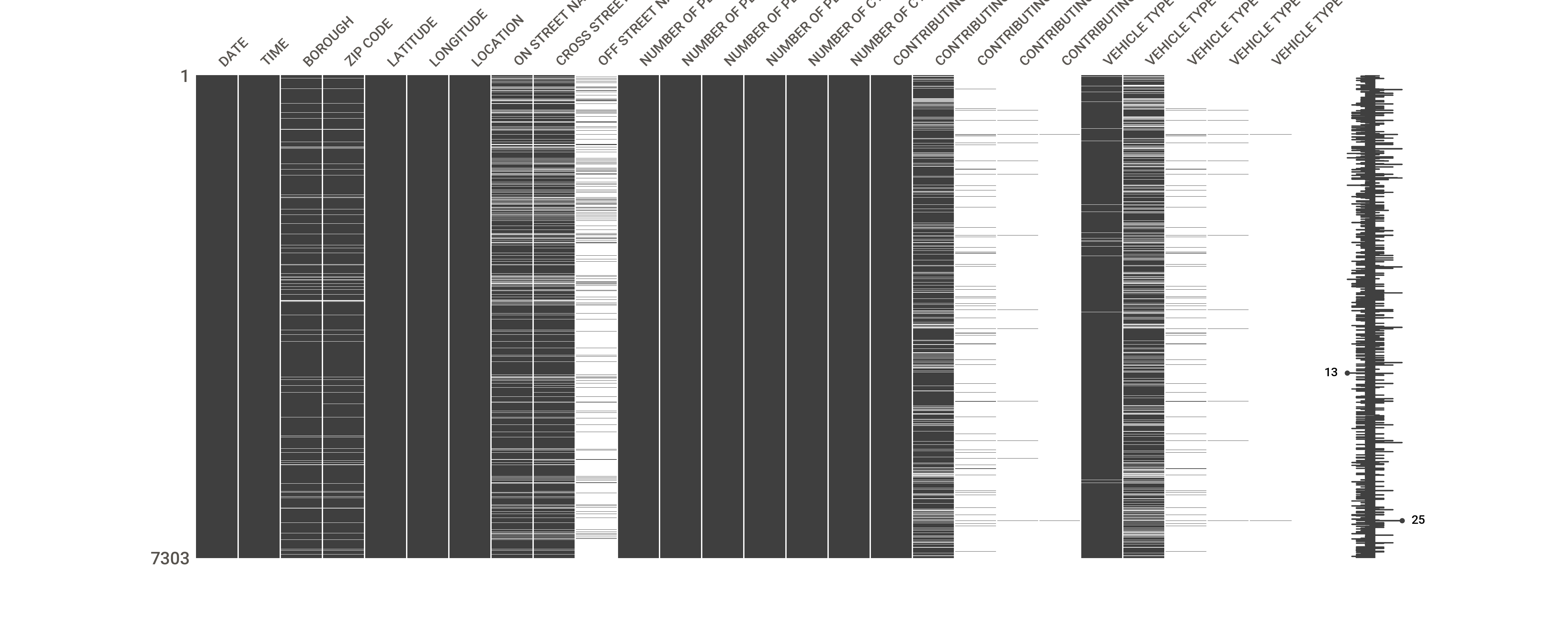
The Missingno Python package has some nice methods to inspect the missing value patterns in data. This is helpful to see the missing value distribution across multiple columns. The matrix() method displays the missing value pattern for the DataFrame.
import missingno as msnomsno.matrix(collisions)
Figure 16.8: Missingness pattern in New York collision data.
Columns without missing values (DATE, TIME) are shown as solid dark bars. Missing values are displayed in white. Figure 16.8 shows the result of matrix() after filling in zeros in the cyclist columns. The sparkline at right summarizes the general shape of the data completeness and points out the rows with the maximum and minimum number of missing values in the data set. At best 11 of the columns have missing values, at worst 23 of the 26 values are missing.
Table 16.3 contains data on property sales. The total value of the property is the sum of the first two columns, the last column is the ratio between sales price and total value. A missing value in one of the first two columns triggers a missing value in the Total column. If either Total or Sales are not present, the appraisal ratio in the last column must be missing.
Table 16.3: Data with column dependencies that propagate missing values.
Land
Improvements
Total
Sale
Appraisal Ratio
30000
64831
94831
118500
1.25
30000
50765
80765
93900
1.16
46651
18573
65224
.
.
45990
91402
137392
184000
1.34
42394
.
.
168000
.
.
133351
.
169000
.
63596
2182
65778
.
.
56658
153806
210464
255000
1.21
51428
72451
123879
.
.
93200
.
.
422000
.
76125
78172
275297
290000
1.14
154360
61934
216294
237000
1.10
65376
.
.
286500
.
42400
.
.
.
.
40800
92606
133406
168000
1.26
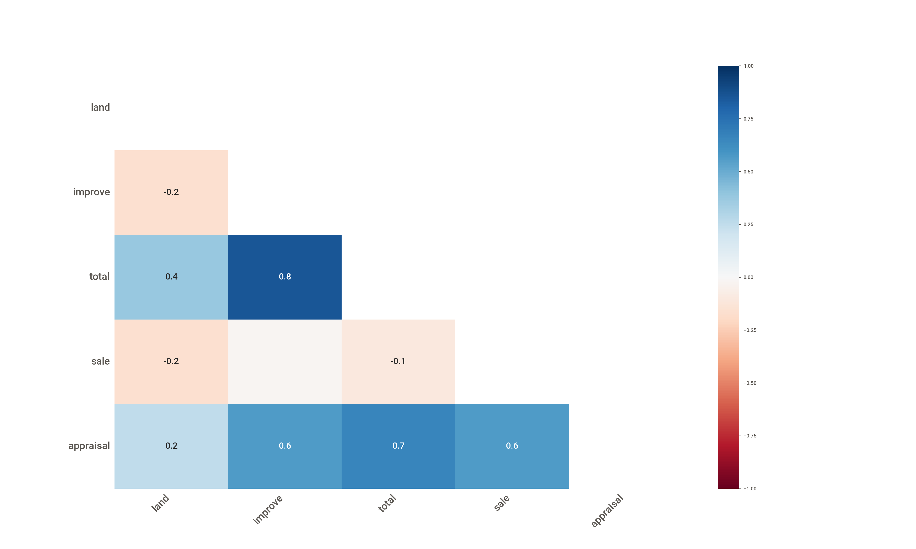
The heatmap() method shows a matrix of nullity correlations between the columns of the data (Figure 16.9).
import duckdbcon = duckdb.connect(database="../ads.ddb", read_only=True)land = con.sql("SELECT * FROM landsales").df()con.close()msno.heatmap(land)
Figure 16.9: Heat map of nullity correlations.
The nullity correlations are Pearson correlation coefficients computed from the isnull() boolean object for the data, excluding columns that are completely observed or completely unobserved. A correlation of –1 means that presence/absence of two variables is perfectly correlated: if one variable appears the other variable does not appear. A correlation of +1 similarly means that the presence of one variable goes together with the presence of another variable. The total is not perfectly correlated with land or improve columns because a null value in either or both of these can cause a null value for the total. Similarly, the large correlations between appraisal and total and between appraisal and sale are indicative that their missing values are likely to occur together.
Data Imputation
In a previous example we used the fillna() method to replace missing values with actual values: the unobserved values for the number of cyclists in the collisions data set were interpreted as no cyclists were injured, replacing NaNs with zeros. This is an example of data imputation, the process of replacing unobserved (missing) values with usable values.
Imputation must be carried out with care. It is tempting to replace absent values with numbers to complete the data: records are not removed from the analysis, the sample size is maintained, and calculations no longer fail. However, imputing values that are not representative introduces bias into the data.
Completing missing values based on information in other columns often seems simple on the surface, but it is fraught with difficulties—there be dragons! Suppose using address information to fill in missing zip codes. It is not sufficient to know that the city is Blacksburg. If we are talking about Blacksburg, SC, then we know the ZIP code is 29702. If it is Blacksburg, VA, however, then there are four possible ZIP codes; we need the street address to resolve to a unique value. Inferring a missing attribute such as gender should never be done. You cannot safely do it using names. Individuals might have chosen to not report gender information. You cannot afford to get it wrong.
If string-type data are missing, and you want to include them into the analysis, you can replace the missing values with an identifying string such as “Unobserved” or “Unknown”. That allows you to break out results for these observations in group-by observations, for example.
Approaches
If you decide to proceed with imputation of missing values based on algorithms, here are some options:
LOCF
The missing value is replaced with the last complete observation preceding it: the last observation is carried forward. It is also called a forward fill. This method requires that the order of the observations in the data is somehow meaningful. If observations are grouped by city, it is probable that a missing value for the city column represents the same city as the previous record, unless the missing value falls on the record boundary between two cities.
Backfill
This is the opposite of LOCF; the next complete value following one or more missing values is propagated backwards.
Mean/Median imputation
This technique applies to numeric data; the missing value is replaced based on the sample mean, the sample median, or other statistical measures of location calculated from the non-missing values in a column. If the data consists of groups or classes, then group-specific means can be used. For example, if the data comprises age groups or genders, then missing values for a numeric variable can be replaced with averages for the variable by age groups or genders.
Interpolation methods
For numerical data, missing values can be interpolated from nearby values. Interpolation calculations are based on linear, polynomial, or spline methods. Using the interpolate() method in pandas, you can choose between interpolating across rows or columns of the DataFrame.
Donor methods
Also called hot-deck imputation, this method relies on finding similar data points or groups of data points to the records with missing values. These points are the donors for the missing value and a donor value is chosen from the set at random, in sequence, or as the donor average. A critical step is selecting the “similar units” that define the set of donors for the missing value. For example, KNNImputer in sklearn uses a K-nearest neighbor method and chooses the donor as an average of the closest neighbors.
Regression imputation
The column with missing values is treated as the target variable of a regression model, using one or more other columns as input variables of the regression. The missing values are then treated as unobserved observations for which the target is predicted.
Matrix completion
Based on principal component analysis (PCA), missing values in an \(r \times c\) numerical array are replaced with a low-rank approximation of the missing values based on the observed values. It is a good method when the variables capture related information.
Generative imputation
If the data consist of images or text and portions are unobserved, for example, parts of the image are obscured, then generative methods can be used to fill in missing pixels in the image or missing words in text.
Surrogate variables
This is the approach built into tree-based methods such a CART and recursive partitioning. The idea is to evaluate at each split point in the tree alternative variables (surrogates) that can be used in case the primary split variable is unobserved. The rpart package in R by default adds up to five surrogate variables for each split variable.
Because trees use surrogate variables, it is sometimes claimed that decision trees and related methods such as random forests, gradient boosting, and extreme gradient boosting handle missing values automatically and that one does not have to worry about missing values with these methods. That is not correct. In using surrogate variables the same caveats apply as with all missing value handling: if the underlying process is not MCAR, then there is potential to bias the results.
Another important consideration is choosing between univariate and multivariate imputation. Univariate imputation considers only the values in a given column to impute missing values. LOCF, backfill, or mean/median imputation are examples. Multivariate imputation considers data from all columns to derive an imputed value. An advantage of multivariate imputation is to draw on (and preserve) the relationships among the columns. That makes sense if the columns represent the same concept. For example, in gene microarray analysis, the columns represent expression of different genes. When the columns represent different concepts it is more difficult to justify combining them: imagine imputing a missing miles per hour data point with an average of horsepower and number of cylinders.
Simple examples
To demonstrate some of these techniques, consider this simple 6 x 3 DataFrame.
import numpy as npimport pandas as pdnp.random.seed(42)df = pd.DataFrame(np.random.standard_normal((6, 3)))df.iloc[:4,1] = np.nandf.iloc[1:3,2] = np.nandf
          0         1         2
0  0.496714       NaN  0.647689
1  1.523030       NaN       NaN
2  1.579213       NaN       NaN
3  0.542560       NaN -0.465730
4  0.241962 -1.913280 -1.724918
5 -0.562288 -1.012831  0.314247
You can choose a common fill value for all columns or vary the value by column.
Missing values in the second column are replaced with 0.3, those in the last column with zero. Forward (LOCF) and backward imputation are available by setting the method= parameter of fillna():
df.fillna(method="ffill")
          0         1         2
0  0.496714       NaN  0.647689
1  1.523030       NaN  0.647689
2  1.579213       NaN  0.647689
3  0.542560       NaN -0.465730
4  0.241962 -1.913280 -1.724918
5 -0.562288 -1.012831  0.314247
Notice that the forward fill does not replace the NaNs in the second column as there is no non-missing last value to be carried forward. The second and third row in the third column are imputed by carrying forward 0.647689 from the first row. With a backfill imputation the DataFrame is fully completed, since both columns have an observed value after the last missing value.
The sample means of the non-missing observations in the second and third columns are -1.463056 and -0.307178, respectively. Imputing with the sample mean has the nice property to preserve the sample mean of the completed data:
df.fillna(df.mean()).mean()
0    0.636865
1   -1.463056
2   -0.307178
dtype: float64
You can use other location statistics than the mean. The following statement imputes with the column-specific sample median:
To demonstrate imputation by interpolation, consider this simple series:
s = pd.Series([0, 2, np.nan, 8])s
0    0.0
1    2.0
2    NaN
3    8.0
dtype: float64
The default interpolation method is linear interpolation. You can choose other method, for example, spline or polynomial interpolation, with the method= option.
     a    b    c     d
0  0.0  NaN -1.0   1.0
1  NaN  2.0  NaN   NaN
2  2.0  3.0  NaN   9.0
3  NaN  4.0 -4.0  16.0
The default interpolation method is linear with a forward direction across rows.
df.interpolate()
     a    b    c     d
0  0.0  NaN -1.0   1.0
1  1.0  2.0 -2.0   5.0
2  2.0  3.0 -3.0   9.0
3  2.0  4.0 -4.0  16.0
Because there was no observed value preceding the missing value in column b, the NaN cannot be interpolated. Because there was no value past the last missing value in column a, the NaN is replaced with the last value carried forward.
To interpolate in the forward and backward direction, use limit_direction=’both’:
     a    b    c     d
0  0.0 -0.5 -1.0   1.0
1  NaN  2.0  2.0   2.0
2  2.0  3.0  6.0   9.0
3  NaN  4.0 -4.0  16.0
Donor imputation with \(K\)-nearest neighbor
Scikit-learn provides a donor-based imputation method with KNNImputer. This function selects donor values to replace missing values based on the \(k\) nearest neighbors of the missing observation. In determining the \(k\) nearest neighbors, the imputer considers values in all available columns with non-missing values. In other words, this is a multivariate imputation method that possibly draws on multiple columns to compute the imputed values.
The advantage of multivariate imputation is to take into account (and preserve) the relationships between the columns. That makes sense in a gene microarray, for example, where the columns represent similar things, the expression of genes. When features represent very different attributes, combining them to impute values might not make sense.
As we can see from the following simple example, whether KNNImputer draws on a single column or multiple columns to find the donor values depends on the missing value pattern and the data.
import numpy as npimport pandas as pd# Create a sample dataset with missing values (NaN)data = {'X1': [10, 12, np.nan, 15, 14],'X2': [5, np.nan, np.nan, 10, 16],'X3': [20, 22, 25, np.nan, 30]}df = pd.DataFrame(data)print("Original DataFrame with missing values:")
Original DataFrame with missing values:
print(df)
     X1    X2    X3
0  10.0   5.0  20.0
1  12.0   NaN  22.0
2   NaN   NaN  25.0
3  15.0  10.0   NaN
4  14.0  16.0  30.0
Notice that a single value is missing for X1 and X3 and that two values are missing for X2. Also, notice that observation 2 has missing values in two columns.
To use KNNImputer we need to choose the number of nearest neighbors from which to derive the imputed value. The default is n_neighbors=5. By default, distances between observations are calculated as Euclidean distance. To show how KNN imputation works, and because the data set is tiny, we compute imputed values for \(k=1\) and \(k=2\).
from sklearn.impute import KNNImputerimputer1 = KNNImputer(n_neighbors=1) imputer2 = KNNImputer(n_neighbors=2) # Fit the imputer to the data and transform it to impute missing valuesimputed_array1 = imputer1.fit_transform(df)imputed_array2 = imputer2.fit_transform(df)
fit_transform returns a NumPy array, which we turn back into a DataFrame:
df_imputed1 = pd.DataFrame(imputed_array1, columns=df.columns)df_imputed2 = pd.DataFrame(imputed_array2, columns=df.columns)print("\nDataFrame after KNN(1) Imputation:")
For \(k=2\), the imputed value for X1 is the average of the first two observations \[
\widehat{x}_{13} = \frac{x_{11}+x_{12}}{2}=\frac{10+12}{2}=11
\]
\(x_{11}\) and \(x_{12}\) are called the donor values for \(\widehat{x}_{13}\). The imputed value for X3 must be the average of \(x_{32}=22\) and \(x_{35} = 30\) since there is no other way to get a two-value average of \(26\).
The first missing value for X2 is imputed as the average of \(x_{21}=5\) and either \(x_{24} = 10\) or \(x_{11}=10\). The second missing value is imputed as the average of \(x_{21}=5\) and \(x_{21}=16\) or as the average of \(x_{11}=10\) and \(x_{13}=11\) or as the average of \(x_{24}=10\) and \(x_{23}=11\).
Uncertainty accounting
Imputation seems convenient and relatively simple, and there are many methods to choose from. As you can see from this discussion, there are also many issues and pitfalls. Besides introducing potential bias by imputing with bad values, an important issue is the level of uncertainty associated with imputed values.
Unless the data were measured with error or entered incorrectly, you have confidence in the observed values. You cannot have the same level of confidence in the imputed values. The imputed values are estimates based on processes that involve randomness. One source of randomness is that our data represents a random sample—a different set of data gives a different estimate for the missing value. Another source of randomness is the imputation method itself. For example, hot-deck imputation chooses the imputed value based on randomly selected observations with complete data. Matrix imputation is a low-rank approximation. Regression imputation uses a statistical model to predict missing values.
Accounting for these multiple levels of uncertainty is non-trivial. If you pass imputed data to any statistical algorithm, it will assume that all values are known with the same level of confidence. Once the data has been completed by imputation, a random forest or regression routine does not distinguish observed and imputed values—they are just numbers.
There are ways to take imputation uncertainty into account. You can assign weights to the observations where the weight is proportional to your level of confidence. Assigning smaller weights to imputed values reduces their impact on the analysis. A better approach is to use bootstrap techniques to capture the true uncertainty and bias in the quantities derived from imputed data. This is more computer intensive than a weighted analysis but very doable with today’s computing power.
Definition: Bootstrap
To bootstrap a data set is to repeatedly sample from the data with replacement. Suppose you have a data set of size \(n\) rows. \(B\) = 1,000 bootstrap samples are 1,000 data sets of size \(n\), each drawn independently from each other, and the observations in each bootstrap sample are drawn with replacement.
Bootstrapping is a statistical technique to derive the sample distribution of a random quantity by simulation. You apply the technique to each bootstrap sample and average the results.
Using the bootstrap with missing value imputation means to draw \(B\) random samples with replacement of size \(n\) from the data, apply the imputation method to each sample, then perform the complete-case analysis, and measure the variability of model coefficients (or other quantities of interest) across the \(B\) bootstrap samples.
I hope you take away from this discussion that imputation is possible, imputation is not always necessary, and imputation must be done with care.
16.5 Outlier and Anomalies
Is a credit card transaction in the amount of $6,000 an outlier? Well, it depends. For someone whose typical spending pattern is $50–$200 per transactions that is an unusual amount. For a high-income customer or a business it might be a typical transaction amount.
Outliers and anomalies are observations that deviate from a norm or expectation. The difference is that an outlier is an observation that is unusual in value, whereas an anomaly refers to an unusual pattern or behavior. A single extreme observation is an outlier; a group of extreme observation can indicate an anomalous pattern.
Example: ESG Reporting
The ESG (Environmental, Social, and Governance) framework is used to evaluate a company’s sustainability and ethical impact. Suppose a company has historically reported stable carbon emissions. Within the course of a year, it has suddenly reduced its emissions by 25%, without announcing any major changes to its operations.
An emission reduction by 25% might not be an outlier. Other companies might be able to achieve that. Achieving the reduction without changes to operations is an anomaly.
An outlier is simply an unusual observation and what is typical depends on the context and on how we interpret the typical. If we declare observations as outliers, the first reaction should not be to delete the records or to alter the data. For example, an observation can be an outlier with respect to one statistical model but not with respect to another. Outliers are often the most interesting data points that identify a breakdown of the model. Removing them to make the model look better is the wrong approach; change the model, not the data.
If you study human performance and data from exceptional athletes with record-breaking performance is very different from the performance characteristic of the average Joe or Jane, the exceptional data is rare and legitimate. It should be preserved and not deleted.
The approach is different if the outlier is due to invalid values, measurement error, or violates basic business constraints. Clearly, in this case we do not want to contaminate the analysis with bad data. If the value cannot be corrected, then the observation needs to be removed. Identifying unusual values that violate business rules or constraints is straightforward: credit scores cannot be above 850, ambient temperatures are not in the 200 degree Fahrenheit range, and a 25 year old cannot have 40 years of professional experience. We do not worry about such extreme-because-wrong data points in this discussion. We are concerned with data points that are unusual and potentially legitimate.
Classification
Outliers can be classified according to different schemas.
Univariate and multivariate outliers. A univariate outlier is unusual with respect to a single distribution, a multivariate outlier is unusual with respect to a joint distribution. The 25-year old with 20 years of work experience is not unusual with respect to the univariate distributions of age and of work experience. The bivariate combination of the values is highly unusual (impossible?) under the joint distribution of age and work experience. Homes with 10 bedrooms exist and homes with 1,200 ft2 of living space are not unusual either—the combination is highly unusual, however.
Global and local outliers. An outlier is global it if is unusual with respect to all the data. It is a local outlier if it is unusual relative to data in its neighborhood. A temperature reading of 80oF is not unusual globally, but is unusual in Alaska or in Virginia during the winter. A $200,000 house price might be typical nationally but is extremely low in Manhattan.
Contextual (conditional) outliers require additional, contextual, information in addition to the value to judge whether they are usual or unusual. The introductory credit card example of a $6,000 charge is an example. We need to know more about the spending habits of the account. A person’s blood pressure might be high compared to the general population but reasonable given the individual’s medical condition. Extreme website traffic is unusual during off-peak hours but normal during promotion periods.
Collective outliers involve more than one observation. The observations are individually normal but form an anomalous pattern as a group. A small withdrawal from a bank account is normal, but a sequence of such withdrawals in short succession is an unusual pattern that can suggest fraud.
Error-Based outliers result from mistakes in data collection, processing, or transmission. Typographical errors create impossible values, sensor malfunctions produce erroneous readings. These outliers require correction or removal to maintain data quality.
Extreme value outliers fall into the tails of distributions and help understand the boundaries and limits of system behavior. They are valuable for risk assessment (worst-case scenario) and capacity planning.
Detection
From the classification of outliers it is clear that values alone might not be sufficient to determine what observations are unusual. You might need to consult domain experts to determine whether network spikes are signs of a cybersecurity attack, to understand seasonal patterns, or to figure out whether an insurance claim suggests a fraud attempt.
During data engineering we often fall back on purely numerical approaches. By not taking into account context, conditions, joint distributions, and domain expertise, numerical methods alone might miss the big picture.
Z-scores
Z-score analysis is also known as standard score analysis and is simple. The \(z\)-score expresses how many standard deviations an observation is away from the mean of the data. Because the true mean and standard deviation are not known, the sample mean (\(\overline{x}\)) and sample standard deviation \(s_x\) are substiuted. That is the \(z\)-score: \[
z = \frac{x-\overline{x}}{s_x}
\]
Larger values of \(z\) imply more extreme observations. The value of \(z\) is positive if the observation falls to the right of the mean and negative if it lies to the left of the mean.
Before we declare observations as outliers based on the \(z\)-score, we need to take the distributional properties into account. An observation that is 2 standard deviations above the mean may be fairly unusual for a Gaussian distribution, it occurs in 2.2% of all cases. For a Gamma(3,1/2) random variable, a \(z\)-score of 2 occurs in 4.4% of all cases.
For a Gaussian distribution, the percentage of observations with \(z\)-scores of 1, 2, 3, and 4 are
If you sample 10,000 observation from a Gaussian distribution, you should expect around 27 of them to have a \(z\)-score of \(|z| > 3\).
When the data distribution is highly skewed, the \(z\)-score based on the sample mean is sometimes replaced with a score that centers around the median of the sample: \[
z^* = \frac{x-\text{median}_x}{s_{x}}
\]
Box plots and five-number summaries
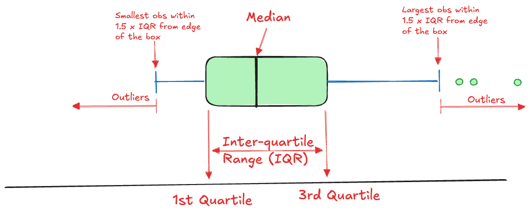
The box plot is one of the most useful visual summaries of a univariate distribution. It combines information about central tendency (location), dispersion, and extreme observations in a single display (Figure 16.10).
Figure 16.10: Schematic of a box plot
The construction of the box plot is based on five summary statistics, sometimes called Tukey’s five-number summary. These are
the lower whisker
the lower hinge of the box (\(Q_1\))
the median (\(Q_2\))
the upper hinge of the box (\(Q_3\))
the upper whisker
The lower and upper whiskers extend to the value of an observation within \(1.5\times \text{IQR}\), where IQR is the inter-quartile range, IQR = \(Q_3 - Q_1\). Any observation that falls outside of the range of the whiskers (above or below) is termed an outlier and shown on the box plot with circles.
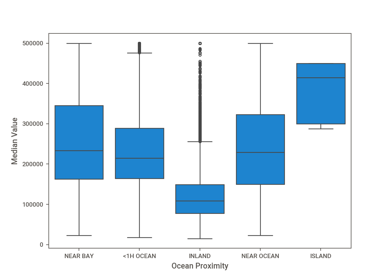
Figure 16.11 displays box plots of the median house value by ocean proximity for the California housing data. By the box plot definition of outlier there are some unusual high house values within one hour of the ocean and many outliers for inland properties, although the majority of the inland properties have lower values compared to the other areas.
import matplotlib.pyplot as pltimport seaborn as snssns.boxplot(x="ocean_proximity", y="median_house_value", data=CA_houses)plt.xlabel("Ocean Proximity")plt.ylabel("Median Value")plt.show()
Figure 16.11: Distribution of median house value by proximity to ocean.
Learning approaches
Unsupervised
We briefly mention unsupervised statistical learning methods for outlier detection here. These methods are discussed more fully in the methods chapters of the Statistical Learning course.
Clustering methods in unsupervised learning group observations based on features into groups such that similarity is greater within the groups than between groups. These groups are referred to as clusters and are formed as a result of the analysis, not a priori.
A \(K\)-nearest neighbors analysis can identify outliers as points whose distance to their \(k\)th nearest neighbor exceeds a threshold, making them suitable for situations where outliers exist in isolation. DBSCAN clustering can simultaneously identify clusters and outliers, marking points that do not belong to any dense region as potential anomalies.
Isolation Forests are a highly efficient method for anomaly detection in large datasets. The method is based on decision trees, it is unsupervised because there is no target variable being predicted or classified. Instead, the data are randomly and repeatedly split. Each tree isolates data points by recursively splitting the data based on randomly selected features and split values. Outliers stand out because they require fewer splits to isolate from the rest of the data—hence the name isolation forest. Based on the average path length across all trees in the forest, the algorithm produces an anomaly score for each data point.
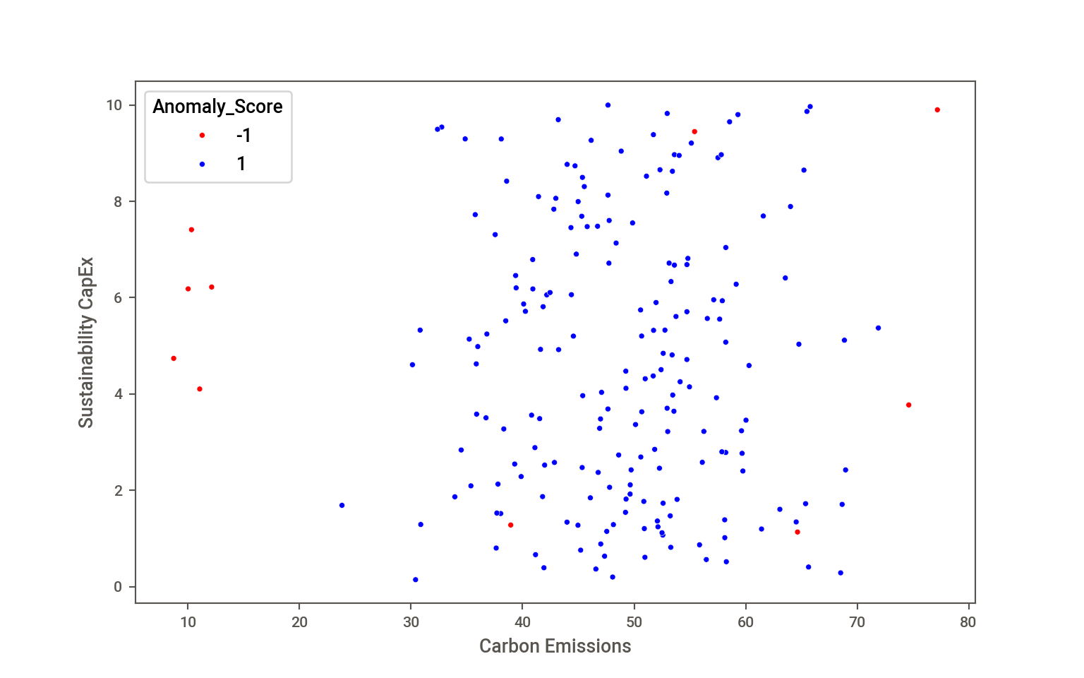
Example: Isolation Forest for ESG Data
This example follows Joury (2025), who examines isolation forests and DBSCAN for anomaly detection with ESG (Environmental, Social, and Governance) data.
The data are simulated carbon emissions, ESG scores, and capital expenditures for sustainability from 200 companies. After simulating the data from Gaussian distributions, the carbon emissions values are randomly perturbed (reduced) without affecting the capital expenditures. Can the isolation forest detect those anomalies?
import numpy as npimport pandas as pdfrom sklearn.preprocessing import StandardScalernp.random.seed(42)n_samples =200data = pd.DataFrame({"Company": [f"Company_{i}"for i inrange(n_samples)],"Carbon_Emissions": np.random.normal(50, 10, n_samples),"ESG_Score": np.random.normal(70, 5, n_samples),"Sustainability_CapEx": np.random.uniform(0, 10, n_samples)})# Introduce anomalies (sudden emissions drop but no investment increase)data.loc[np.random.choice(n_samples, 5, replace=False), "Carbon_Emissions"] *=0.2scaler = StandardScaler()scaled_features = scaler.fit_transform(data.iloc[:, 1:])df_scaled = pd.DataFrame(scaled_features, columns=["Carbon_Emissions", "ESG_Score", "Sustainability_CapEx"])
5 of the 200 observations have a reduction in carbon emissions of 20% without change in sustainability expenditures. This is a proportion of 0.025 of the samples. The contamination parameter of the IsolationForest in sklearn specifies the proportion of outlier contamination in the data and defines the threshold on the scores of the samples.
Well, that is kinda strange. I have to know the proportion of outliers before performing the analysis that identifies the outliers? Think of the contamination rate as a threshold for the suspected outlier proportion. You can use \(z\)-scores or boxplots to get an idea of the relative frequency of outliers. Or analyze historical data or call on the experience of domain experts to determine the hyperparameter. The outlier proportion acceptable to the business is another method for determining this parameter. Since the method is unsupervised, there is no cross-validation available for the hyperparameter. It is a threshold, not the ultimate proportion of detected outliers. You can also leave the contamination parameter unspecified; it defaults to contamination='auto',determining the threshold as in the original paper bei Liu, Ting, and Zhou (2008).
Figure 16.12: Anomaly Detection in ESG Data (Isolation Forest).
The isolation forest flags 10 observations as anomalies with respect to carbon emissions and sustainability expenditures.
Supervised
Support vector machines (SVM) are used to classify observations based on a learned classification rule. Typically they are applied to situations with a two-level (binary) target variable. A variation, one-class SVM, learns a classification boundary that separates “normal” from unusual observations. SVMs in general belong to the supervised learning techniques, one-class SVM is an unsupervised technique as observations do not need to be labeled normal/unusual prior to analysis.
In time series analysis anomalies are assessed relative to moving averages or smoothed series that establish the baseline trends. Dramatic shifts in time series can be analyzed with change point detection algorithms.
Liu, Fei Tony, Kai Ming Ting, and Zhi-Hua Zhou. 2008. “Isolation Forest.” In 2008 Eighth IEEE International Conference on Data Mining, 413–22. https://doi.org/10.1109/ICDM.2008.17.