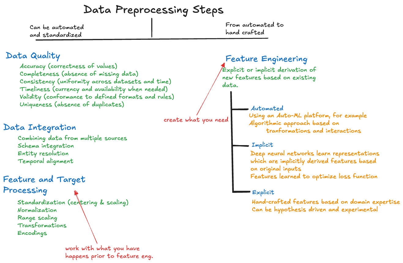
Feature processing is a data preprocessing step, along with data quality, data cleaning, and data integration (Figure 28.1). It is often automated, performed as part of data pipelines. The goal is to get data ready for processing in data science (machine learning, statistical) models; transforming the data into a form that is suitable for analytic processing.
Figure 28.1: Data preprocessing steps. Click to enlarge.
Feature engineering, while technically also a data preprocessing step, is discussed in Chapter 29. It is part of preprocessing because the features are developed (engineered) prior to modeling. However, practitioners think of feature engineering as a more strategic task that requires domain expertise and experimentation and cannot be automated. Having said that, automated feature engineering, so-called AutoML tools and platforms, are available.
Feature processing applies standard transformations such as scaling, normalization, encodings for qualitative variables and text, and distributional transformations to stabilize variance or achieve symmetry. Feature engineering is a creative process of designing and constructing new features from existing data. It requires domain expertise and insight to create meaningful new variables. Examples include creating interaction terms between variables, extracting time-based features from time stamps, aggregating transaction data into spending patterns, or combining multiple raw features into derived metrics.
In Chapter 16 the concern was with profiling and cleaning data, removing duplicate values, handling missing values, etc. Chapter 19 discussed the basics of combining data from multiple sources. The goal was that the data have the appropriate quality and consistency for any subsequent analysis.
To make the difference between processing for data quality and feature processing explicit, consider the data in Table 28.1.
Table 28.1: City names before and after data processing for quality and after feature processing.
Before Quality Processing
After Quality Processing
\(X_1\)
\(X_2\)
\(X_3\)
New York
New York
1
0
0
NY
New York
1
0
0
new York
New York
1
0
0
LA
Los Angeles
0
1
0
LAX
Los Angeles
0
1
0
Los Ang.
Los Angeles
0
1
0
Chicago
Chicago
0
0
1
Chicago, Ill.
Chicago
0
0
1
Data quality ensures that city names are consistent in the data set. Feature processing transforms the consistent city names into a numerical representation for analytic processing, the features \(X_1\), \(X_2\), and \(X_3\). The features encode the possible values of the city variable in numerical values. Because there are three cities, three binary variables are created, a process called one-hot encoding.
Preprocessing data for modeling applies to the target variable and the input variables. For example, one-hot encoding of categorical variables is used to represent categorical input variables as multiple dummy variables on the right hand side of the model. It is also used to encode categorical target variables for classification models.
28.2 Standardization
Centering and Scaling
Standardizing a variable \(X\) comprises two steps, centering and scaling. Scaling does what it says, it replaces \(x_i\) with \(c\times x_i\) where \(c\) is the scaling factor. Centering means shifting the variable so that it is centered at some specific value. The common parameters of standardization are centering at the mean \(\overline{x}\) and scaling with the standard deviation \(s_x\): \[
z = \frac{x-\overline{x}}{s_x}
\] The transformed variable has a sample mean of 0 and a sample standard deviation of 1: \[
\overline{z} = 0 \qquad s_z = 1
\]
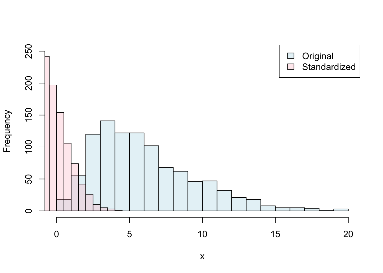
Figure 28.2 shows the effect of standardization of 1,000 observations drawn from a Gamma(3,2) distribution. Centering shifts the data to have mean zero and compresses the dispersion of the data to a standard deviation of one.
Figure 28.2: Original and standardized data drawn from a Gamma(3,2) distribution.
The mean (center) of the original data is 6.0219 and the scale applied by scale() is 3.4536. This is the usual standard deviation calculation based on \(n-1\) as the denominator.
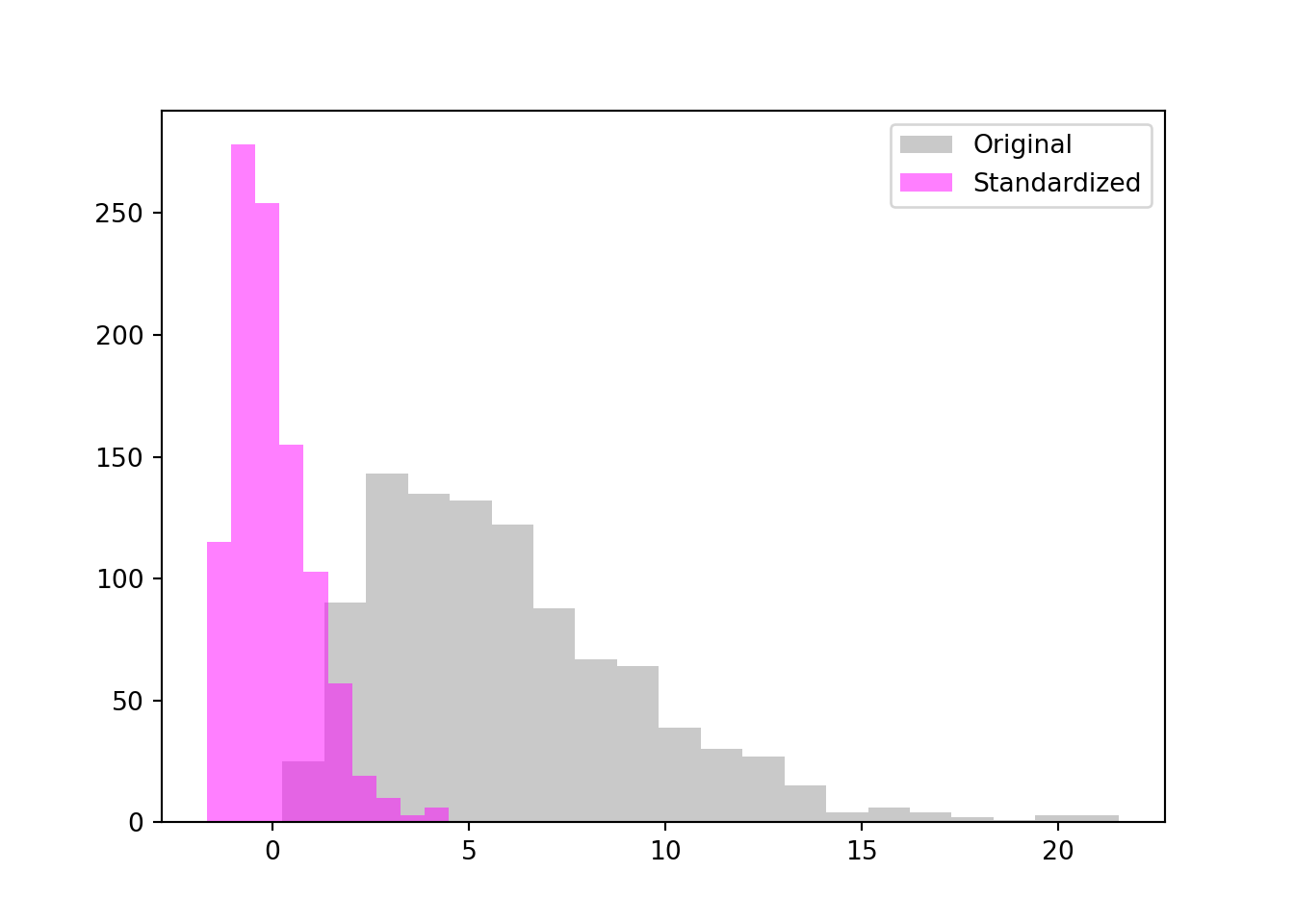
Figure 28.3 shows the effect of standardization of 1,000 observations drawn from a Gamma(3,2) distribution. Centering shifts the data to have mean zero and compresses the dispersion of the data to a standard deviation of one.
import numpy as npfrom sklearn import preprocessingimport matplotlib.pyplot as pltnp.random.seed(234)x = np.random.gamma(shape=3,scale=2,size=1000)x = np.reshape(x,(-1,1))stder = preprocessing.StandardScaler().fit(x)stder.mean_
Figure 28.3: Original and standardized data drawn from a Gamma(3,2) distribution.
The mean (center) of the original data is 6.021 and the scale applied by StandardScaler is 3.471. Note that this standard deviation calculation is based on np.std() which by default uses \(n\) instead of \(n-1\) as the denominator–using \(n\) instead of \(n-1\) in the calculation of a sample variance yields a biased estimator of the population variance.
Scaling called Standardization
You will find references in the literature and in software documentation to “scaling the data”. It is often understood to mean standardization of the data, that is, centering and scaling.
Be also aware of the default behavior of software packages. The prcomp function for principal component analysis in R, for example, centers the data by default but does not scale by default. The loess function in R normalizes the predictor variables, using scaling to a robust estimate of the standard deviation, but only if there is more than one predictor. The glmnet::glmnet function standardizes the inputs by default (standardize=TRUE) and reports the results on the original scale of the predictors.
Another form of standardization \[
x_i^* = \frac{x_i-\overline{x}}{\sqrt{SS_{x}}}
\] where \(SS_{x}\) is the (mean-corrected) sum of squares of the \(x_i\): \[
SS_{x} = \sum_{i=1}^n (x_i-\overline{x})^2
\] By virtue of centering with the sample mean, the mean of \(x^*\) is zero and the standard deviation is \(1/\sqrt{n-1}\). Also note that variables so centered and scaled have \(\sum (x_i^*)^2 = 1\); they have unit length with respect to the \(L_2\) norm. Finally, this method of standardization is convenient in regression models. You can easily show that the cross-product of two variables standardized in this way equals their Pearson correlation coefficient: \[
\sum_{i=1}^n x_i^* y_i^* = \frac{SS_{xy}}{\sqrt{SS_x \ SS_y}}=r_{xy}
\]
Range Scaling
This form of scaling of the data transforms the data so it falls between a known lower and upper bound, often 0 and 1. Suppose that \(\text{min}(X) \le X \le \text{max}(X)\)
and we want to create a variable \(z_{\text{min}} \le Z \le z_{\text{max}}\) from \(X\). \(Z\) can be computed by scaling and shifting a standardized form of \(X\): \[
\begin{align*}
x^* &= \frac{x-\min(x)}{\max(x)-\min(x)} \\
z &= z_{\text{min}} + x^* \times (z_{\text{max}} - z_{\text{min}})
\end{align*}
\]
In R, you can use the preProcess function in the caret package, along with the predict function. It can operate on all columns of a matrix or data frame, ignoring non-numerical columns. You pass the return object from preProcess to the predict function to generate a data frame from an input data frame.
The following code scales the Gamma(3,2) sample to lie between 0 and 2. Because preProcess operates on matrices or data frames, the vector x is first converted to a data frame.
An advantage of range scaling is that the same range can be applied to training and test data. This makes it easy to process test data prior to applying a model derived from range-scaled data.
To Scale or not to Scale
Some data scientists standardize the data by default. When should you standardize and when should you not? Analytic techniques that depend on measures of distance to express similarity or dissimilarity between observations, or that depend on partitioning variability, typically benefit from standardized input variables.
Examples of the former group are \(K\)-means clustering and hierarchical clustering. Here, the data are grouped into clusters based on their similarity, which is expressed as a function of a distance measure. Without scaling the data, large items tend to be further apart than small items, distorting the analysis toward inputs with large scale. Whether lengths are measured in meters, centimeters, or inches should not affect the analysis. Principal component analysis (PCA) is an example of a method in the second group, apportioning variability to linear combinations of the input variables. Without scaling, inputs that have a large variance can dominate the PCA to the point of not being interpretable or meaningful. Larger things tend to have larger variability compared to small things.
Binary variables are usually not scaled. This includes variables derived from encoding factor variables, see Section 28.4.1.
Train and Test Data
Any preprocessing steps such as standardization, scaling, normalization, are applied separately to train and test data set. In the case of standardization, for example, it means that you split the data into train and test data sets first, then standardize each separately. The training data set is centered and scaled by the means and sample standard deviations in the training data set. The test data set is centered and scaled by the means and standard deviations in the test data set. Both data sets thus have the same properties of zero mean and standard deviation one.
If we were to standardize first and split into training and test data set second, neither data set would have zero mean and unit standard deviation. Furthermore, information from the training data (the mean and standard deviation) would leak into the test data set.
If we were to apply the means and standard deviations from the training data to center and scale the test data, then the test data would not have zero mean and unit standard deviation and information from the training data would also leak into the test data set.
28.3 Normalization
Normalization is sometimes (often, actually) described as a transformation of data to normality; the transformed data appears Gaussian distributed. This is not what we consider normalization here. A variable \(z\) that is normalized with respect to the \(L_2\) norm has the property \[
||\textbf{z}|| = \sqrt{\sum_{i=1}^n z_i^2} = 1
\]
A variable \(x\) can be normalized with respect to any norm by dividing each value by the norm of the vector. In the case of \(L_2\), \[
z_i = \frac{x_i}{||\textbf{x}||}
\]
Normalization is a special case of scaling so that the resulting vector has unit length with respect to some norm. Any norm can be used to normalize the data, for example, the \(L_1\) norm \(|\textbf{x}|\). Note that scaling by the standard deviation does not yield a vector with unit length, but a vector with unit standard deviation.
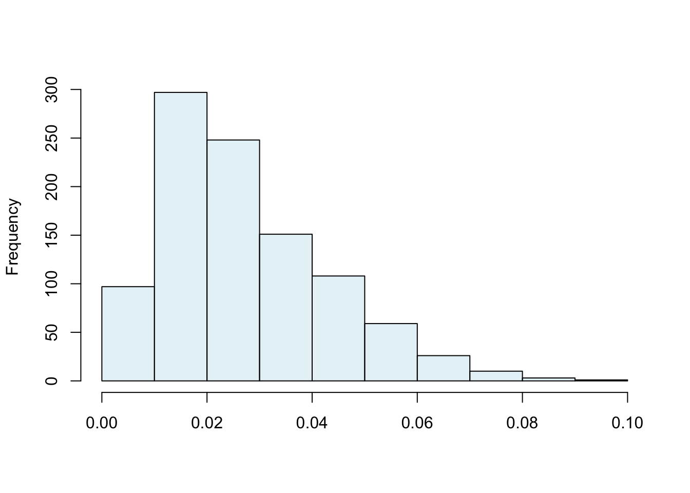
The following code normalizes the Gamma(3,2) sample with respect to \(L_2\).
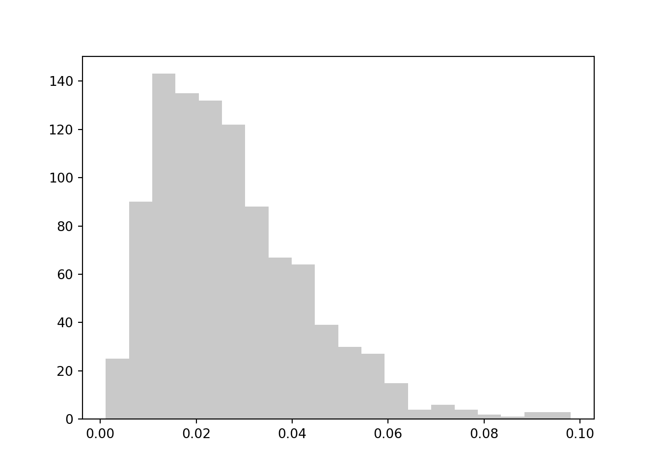
Figure 28.5: Normalized data from the Gamma(3,2) distribution.
Normalization of the sample from the Gamma(3,2) distribution maintains the general shape of the distribution and changes its scale (Figure 28.5).
28.4 Encoding
Data processed by algorithms are represented as numbers, integers and real numbers. The information we collect is often not in the form that can be directly processed by a data science algorithm. Treatments in an experiment could be identified with numeric values, “1”, “2”, “3”, etc. We need to somehow tell the algorithm that these are simply identifying labels and should not be treated as numbers for which differences are meaningful. Treatment “2” is simply different from treatment “1”, it is not necessarily twice as much as treatment “1”. Whether the treatments are labeled “1”, “2”, “3”, or “A”, “B”, “C”, the same analysis must result. A zip code is represented by a numerical label, e.g., 24060 for a region in Blacksburg, VA. It would be silly to treat this as an actual number in an analysis–it is just a label.
Many pieces of information come to us as in the form of character strings, either as structured or as unstructured text. A case of structured text data is when we use strings as labels for things. The treatment labels “A”, “B”, “C” are an example. An example of unstructured text is free-form text such as the quote
The strength of a bureaucracy is measured by its ability to resist change.
An algorithm that predicts the sentiment of the quote must translate these characters into a numerical representation. The process of transforming data from a human-readable form into a machine-readable form is known as encoding in machine learning. The reverse, translating from a machine-readable to a human-readable representation is known as decoding.
In this section we take a somewhat broader view of data encoding.
Definition: Data Encoding and Decoding
Encoding of data is the process of translating information into a numerical format for processing by a statistical or machine learning algorithm.
Decoding is translating information from the numerical format used in analytic processing back into human-readable form.
Encoding is more important to us at this stage. When dealing with natural language processing tasks such as sequence-to-sequence modeling, encoding and decoding are important. An example is the translation of text from one language into another using artificial neural networks. The input text is encoded into numeric format, processed by a network, and the output of that network is decoded by another network into the target language of translation.
Factor Variables
The first case of encoding information is the processing of factor input variables. Factors are categorical variables representing levels (or classes, or categories, or states). For example, the variable treatment with levels “A”, “B”, and “C” is a three-level factor. When this variable is used in a statistical model, it enters the model through its levels, not through its values. That is why some software refers to the process of encoding factor variables as levelization.
To encode factor variables, three decisions affect the representation of the variable and the interpretation of the results:
The order of the levels
The method of encoding
The choice of reference level—if any
The order of the levels is important because it affects the order in which the factor levels enter the model and how the \(\textbf{X}\) matrix is constructed. Consider the following example, which we will use throughout this section, of two factors A and B with 2 and 3 levels, respectively, and a numeric variable \(X\).
Table 28.2: Data with target \(Y\), two factors \(A\) and \(B\) with 2 and 3 levels, respectively, and a numeric input variable \(X\). To distinguish the values of the variables from subsequent encodings, the values are shown in boldface.
Y
A
B
\(X\)
1
1
1
1
2
1
2
0.5
3
1
3
0.25
4
2
1
1
5
2
2
0.5
6
2
3
0.25
One-hot encoding
One-hot encoding, also called standard encoding or dummy encoding, transforms the \(k\) levels of a factor into \(k\) columns of 0/1 values (dummy variables). The value in the \(j\)th dummy variable is 1 if the factor is at level \(j\), 0 otherwise. The one-hot encoding for \(A\) and \(B\) in Table 28.2 is shown in Table 28.3.
Table 28.3: One-hot encoding of \(A\) and \(B\).
A
\(A_1\)
\(A_2\)
B
\(B_1\)
\(B_2\)
\(B_3\)
1
1
0
1
1
0
0
1
1
0
2
0
1
0
1
1
0
3
0
0
1
2
0
1
1
1
0
0
2
0
1
2
0
1
0
2
0
1
3
0
0
1
\(A_1\) and \(A_2\) are the first and second columns of the encoded 2-level factor \(A\). So why does the order in which these columns enter a statistical model matter? Suppose our model is a linear model with inputs \(X\), a numeric variable, and \(A\) (\(\textbf{x} = [x, A_1, A_3]\)): \[
f(\textbf{x}) = \beta_0 + \beta_1x + \beta_2 A_1 + \beta_2 A_2
\] For the six observations in Table 28.2, the \(\textbf{X}\) matrix of the model is \[
\textbf{X} = \left [\begin{array}{rrrr}
1 & 1 & 1 & 0 \\
1 & 0.5 & 1 & 0 \\
1 & 0.25 & 1 & 0 \\
1 & 1 & 0 & 1 \\
1 & 0.5 & 0 & 1 \\
1 & 0.25 & 0 & 1 \\
\end{array} \right]
\] There is a problem, the first column of \(\textbf{X}\) is the sum of the third and forth column. This perfect linear dependency makes the \(\textbf{X}\) matrix singular, the \(\textbf{X}^\prime\textbf{X}\) matrix cannot be inverted, and the ordinary least squares solution cannot be computed.
To remedy this problem many software packages implicitly make one of the levels of a one-hot encoded factor a reference level. For example, R takes the first level of a factor as the reference level. The following code creates a data frame from the data in Table 28.2, declares the numeric variable A as a factor and assigns the second level as the reference level.
df <-data.frame(y=c(1,2,3,4,5,6),x=c(1,0.5,0.25,1,0.5,0.25),A=c(1,1,1,2,2,2))df$A <-relevel(as.factor(df$A),ref=2)coef(summary(lm(y ~ x + A, data=df)))
             Estimate Std. Error   t value     Pr(>|t|)
(Intercept)  6.500000  0.2089277  31.11124 7.296355e-05
x           -2.571429  0.2857143  -9.00000 2.895812e-03
A1          -3.000000  0.1781742 -16.83746 4.561983e-04
The analysis now succeeds but the coefficients reported seem to be for a model without the reference level, namely \[
f(\textbf{x}) = \beta_0 + \beta_1x + \beta_2 A_1
\]
You can easily verify by specifying this model directly:
df2 <-data.frame(y=c(1,2,3,4,5,6),x=c(1,0.5,0.25,1,0.5,0.25),A1=c(1,1,1,0,0,0))coef(summary(lm(y ~ x + A1, data=df2)))
             Estimate Std. Error   t value     Pr(>|t|)
(Intercept)  6.500000  0.2089277  31.11124 7.296355e-05
x           -2.571429  0.2857143  -9.00000 2.895812e-03
A1          -3.000000  0.1781742 -16.83746 4.561983e-04
So where did the information about \(A_2\) end up? To see how this works, consider the model formula for the cases \(A_1 = 0\) and \(A_1 = 1\):
But the value \(A_1=0\) corresponds to \(A_2 = 1\). The simple linear regression \(\beta_0 + \beta_1 x\) is the response for the case where \(A_2 = 1\). The coefficient \(\beta_2\) now measures the difference between the two levels of \(A\), with \(A = 2\) serving as the reference level. The model has two intercepts, one for \(A=1\), and one for \(A=2\), their values are \(6.5 - 3 = 3.5\) and \(6.5\), respectively.
You can also see this from the coefficient estimate in the R output: the sample mean of \(Y\) when \(A = 1\) is \(\overline{y}_{A=1} = 3\) and \(\overline{y}_{A=2} = 6\). Their difference is \(\widehat{\beta}_2 = -3\).
If the first level is chosen as the reference level, this estimate has the opposite sign:
df <-data.frame(y=c(1,2,3,4,5,6),x=c(1,0.5,0.25,1,0.5,0.25),A=c(1,1,1,2,2,2))df$A <-relevel(as.factor(df$A),ref=1)coef(summary(lm(y ~ x + A, data=df)))
             Estimate Std. Error  t value     Pr(>|t|)
(Intercept)  3.500000  0.2089277 16.75220 0.0004631393
x           -2.571429  0.2857143 -9.00000 0.0028958122
A2           3.000000  0.1781742 16.83746 0.0004561983
\(A=1\) now serves as the reference level and the coefficient associated with A2 is the difference between the intercept at \(A=2\) and at \(A=1\). The absolute intercepts of the two level remain the same, \(3.5\) for \(A=1\) and \(3.5 + 3 = 6.5\) for \(A=2\).
When a factor has more than two levels, reference levels in one-hot encoding works the same way, the effects of all levels is expressed as the difference of the level with respect to the reference level.
Caution
If a statistical model contains factors and you interpret the coefficient estimates you must make sure to understand the encoding method–including level ordering and reference levels—otherwise you might draw wrong conclusions about the effects in the model. When making predictions, the choice of order and reference level does not matter, predictions are invariant, as you can easily verify in the example above.
The issue of a singular cross-product matrix \(\textbf{X}^\prime\textbf{X}\) could have been prevented in the model with \(X\) and \(A\) by dropping the intercept. This model has a full-rank \(\textbf{X}\) matrix \[
\textbf{X} = \left [\begin{array}{rrr}
1 & 1 & 0 \\
0.5 & 1 & 0 \\
0.25 & 1 & 0 \\
1 & 0 & 1 \\
0.5 & 0 & 1 \\
0.25 & 0 & 1 \\
\end{array} \right]
\]
Even without an intercept, the problem resurfaces as soon as another factor enters the model. Suppose we now add \(B\) in one-hot encoding to the model. The \(\textbf{X}\) matrix gets three more columns:
\[
\textbf{X} = \left [\begin{array}{rrrrrr}
1 & 1 & 0 & 1 & 0 & 0\\
0.5 & 1 & 0 & 0 & 1 & 0\\
0.25 & 1 & 0 & 0 & 0 & 1\\
1 & 0 & 1 & 1 & 0 & 0\\
0.5 & 0 & 1 & 0 & 1 & 0\\
0.25 & 0 & 1 & 0 & 0 & 1\\
\end{array} \right]
\] Again, we end up with perfect linear dependencies among the columns. The sum of columns 2–3 equals the sum of columns 4–6. It is thus customary to not drop the intercept when factors are present in the model.
Average effect encoding
An encoding that avoids the singularity issue creates only \(k-1\) columns from the \(k\) levels of the factor and expresses the effect of the levels as differences in the effects from the average effect across all levels. This encoding also relies on the choice of a reference level. Suppose we apply average effect encoding to \(B\) and choose \(B=3\) as the reference level.
Average effect encoding for \(B\) with reference level \(B=3\).
B
\(B_1\)
\(B_2\)
1
\(1\)
\(0\)
2
\(0\)
\(1\)
3
\(-1\)
\(-1\)
1
\(1\)
\(0\)
2
\(0\)
\(1\)
3
\(-1\)
\(-1\)
Baseline encoding
In this encoding, \(k-1\) columns are created for the \(k\) levels of the factor. The first level is taken as the baseline and the effects are expressed in terms of differences between successive levels. Baseline encoding of \(B\) results in the following encoding:
Baseline encoding for \(B\) with reference level \(B=3\).
B
\(B_1\)
\(B_2\)
1
\(0\)
\(0\)
2
\(1\)
\(0\)
3
\(1\)
\(1\)
1
\(0\)
\(0\)
2
\(1\)
\(0\)
3
\(1\)
\(1\)
Example: Baseline and Average Encoding
For our little data set, we compute the baseline and average effect encoding here. Before doing so, let’s fit a model with factor \(B\), and without intercept. The coefficients associated with \(B\) are the raw effects of the three levels of \(B\). The intercept is automatically added in model formula expressions in R. You can remove it with -1 from the model.
The (Intercept) of this model represents the level \(B=1\), X1 is the difference of level \(B=2\) to level \(B=1\) and X2 measures the difference between \(B=3\) and \(B=2\).
If \(B\) is expressed in average effect encoding we obtain the following:
X <-matrix(c(1,0,-1,1,0,-1,0,1,-1,0,1,-1),nrow=6,ncol=2)modB_ave_eff <-lm(df$y ~ X)coef(summary(modB_ave_eff))
We see from the initial analysis that the average effect of \(B\) is \(1/3 \times (2.5+3.5+4.5) = 3.5\). The (Intercept) estimate represents this average in the average effect encoding. X1 and X2 represent the differences of \(B=1\) and \(B=2\) from the average. If we place the \(-1\) row at level \(B=2\), then X1 and X2 are the differences of \(B=1\) and \(B=3\) from the average effect of \(B\):
X <-matrix(c(1,-1,0,1,-1,0,0,-1,1,0,-1,1),nrow=6,ncol=2)modB_ave_eff <-lm(df$y ~ X)coef(summary(modB_ave_eff))
Why would you encode continuous variables, that are already in numerical form?
Suppose you are modeling a target as a function of time and the measurements are taken in minute intervals. Maybe such a granular resolution is not necessary and you are more interested in seasonal or annual trends. You can convert the time measurements easily into months, seasons, or years, using date-time functions in the software. Should you now treat the converted values as continuous measurements or as categories of a factor?
When working with age variables we sometimes collect them into age groups. Age groups 0-9 years, 10-24 years, and 25-40 years are not evenly spaced and are no longer continuous. Age has been discretized into a factor variable. Other terms used for the process of discretizing continuous variables are binning and quantizing.
The advantage of using factors instead of the continuous values lies in the introduction of nonlinear relationships while maintaining interpretability. If you model age as a continuous variable, then \[
Y = \beta_0 + \beta_1 \text{age} + \cdots + \epsilon
\] implies a linear relationship between age and the target. Binning age into three groups, on the other hand, leads to the model \[
Y = \beta_0 + \beta_1\text{[Age=0-9]} + \beta_2\text{[Age=10-24]} + \beta_3\text{[Age=25-40]} + \cdots + \epsilon
\] This model allows for different effects in the age groups.
To bin continuous numeric variables in R you can use the cut() function in the base package or the ntile function in dplyr. ntile is a rough ranking of the \(n\) observations from smallest to largest, and then bucketing into k groups of roughly equal size. cut takes a numeric vector and also bins it into k groups of equal width. You can supply a a vector of break points to cut which makes it a good choice to bin values by, say, quantiles of the distribution.
The following code bins the variable x into 5 categories using ntile. The result of the operation is an integer that indicates which category (from smallest to largest) the observation belongs to.
cut creates by default character labels that indicate the lower and upper value of the bins. Setting labels=FALSE results in integer values for the categories
The results of ntile and cut are very different: ntile divides the range of X into intervals of equal number of observations, whereas cut divides the range into intervals of equal width.
You can make cut use equal number of observations by supplying a vector of breaks that corresponds to percentiles of the distribution of the data.
The function KBinsDiscretizer in sklearn.preprocessing bins vectors and matrices of continuous variables using different encoding methods. encode='ordinal' returns a vector or matrix of integers identifying the bin a value belongs to. The default binning strategy (strategy='quantile') is to form bins that contain the same number of points.
encode='onehot-dense' returns a dense matrix of one-hot encoded variables. The following code uses the uniform binning strategy in which all bins have the same widths.
If the values of a variable are structured text in the sense that the values are a limited number of single character strings, the previous encoding methods apply. An example is names of U.S. states or cities, names of active ingredients, medications, places, and so on.
When text is unstructured, it can vary in length and content. How can we encode a sentence such as
The strength of a bureaucracy is measured by its ability to resist change.
The encoding itself is just one of possibly many steps in structuring unstructured data.
Parsing and tokenization breaks unstructured text into smaller units (tokens) for further analysis. A token can be a word, a punctuation symbol, an n-gram such as “Covid 19 pandemic”. Entity recognition finds named entities such as places, persons, businesses in text data. Feature extraction pulls relevant characteristics and attributes from text data and forms numeric columns from it. For example, feature extraction finds temperature or precipitation values in weather reports. Normalization transforms unstructured data into a standardized format, removes duplicates, applies consistent rules to spelling, capitalization, etc.
After all that, suppose we have some unstructured data that needs to be encoded.
One-hot encoding
One-hot encoding can be applied to unstructured text as well, but now it is not immediately obvious how many levels to apply in the encoding. Typically, the unstructured text is compared to a dictionary of tokens. The dictionary can be made up of the tokens found in the text to be encoded, or comprise a larger corpus of text. Clearly, dictionaries tend to be large and one-hot encoding of text leads to data matrices with many columns.
If the dictionary has 10,000 entries, each word or token is represented by a 10,000-element vector that contains 9,999 zeros and a single one that matches the position of the word in the dictionary. This leads to very high-dimensional problems that are also very sparse.
To avoid those problems it is popular to represent words in a lower-dimensional space of real numbers. In other words, rather than choosing 9,999 zeros and a single 1 to represent a particular word, we might choose a 20-dimensional vector of real numbers. This technique is known as word embedding.
Word embeddings
Word embeddings encode words in a low-dimensional space as real-valued vectors. A big advantage of embeddings is that they can be pre-trained and they can capture semantic and syntactic information. Words with similar meaning should have similar representation in the vector space. The distance between two embedding vectors can then be used to measure the similarity between text expressions.
One of the most common embeddings is Word2Vec, developed by Google. It measures the semantic similarity of words based on cosine similarity of the embedding vector. Cosine similarity between two \((n \times 1)\) vectors \(\textbf{a}\) and \(\textbf{b}\) is the cosine of their angle, \[
\cos(\theta) = \frac{\sum_{i=1}^n a_i b_i}{\sqrt{\sum_{i=1}^n a_i^2}\sqrt{\sum_{i=1}^n b_i^2}}
\] A cosine similarity of \(1\) indicates complete similarity, \(0\) indicates lack of correlation, and \(-1\) indicates complete dissimilarity.
Word2Vec is based on two types of neural network models, a continuous bag-of-word (CBOW) model and a skip-gram model. The following Python code trains Word2Vec on a sequence of quotes about change and generates embeddings of length 20. In practical applications the corpus of text you train the model on is much larger, the size of the embedding is 100 or more. You can also download existing Word2Vec embeddings and use those instead of training your own.
from gensim.models import Word2Vecimport gensimimport nltkfrom nltk.tokenize import sent_tokenize, word_tokenize, punkt s ="The strength of a bureaucracy is measured by its ability to resist change.\nThe only constant is change."s = s +"Change is the law of life. And those who look only to the past or present are certain to miss the future\n"s = s +"To improve is to change; to be perfect is to change often\n"s = s +"Change before you have to\n"s = s +"Not everything that is faced can be changed, but nothing can be changed until it is faced\n"s = s +"People who are crazy enough to think they can change the world are the ones who do"f = s.replace("\n", " ")data = []# iterate through each sentence to tokenize the sentencefor i in sent_tokenize(f): temp = []for j in word_tokenize(i): temp.append(j.lower()) data.append(temp)# Create and train a continuous bag-of-words modelmodel1 = gensim.models.Word2Vec(data, min_count=1, vector_size=20, window=5)print(model1.wv["strength"])
print("Cosine similarity between 'strength' and 'ability' - Skip Gram : ",
      model2.wv.similarity('strength', 'ability'))
Cosine similarity between 'strength' and 'ability' - Skip Gram : 0.043875016
print("Cosine similarity between 'strength' and 'change' - Skip Gram : ",
      model2.wv.similarity('strength', 'change'))
Cosine similarity between 'strength' and 'change' - Skip Gram : 0.19225661
28.5 Transforming the Target
The previously discussed preprocessing steps can be applied to any variable, input or target variable.
The purpose of transforming the target variable is to meet distributional assumptions of the analysis. For example, many statistical estimators have particularly nice properties when the data are Gaussian distributed. A common transformation of \(Y\) is thus to morph its distribution so that the transformed \(Y^*\) is closer to Gaussian distributed than \(Y\). Sometimes transformations just aim to create more symmetry or to stabilize the variance across groups of observations. Transformations change the relationship between (transformed) target and the inputs, it is common to transform targets to a scale where effects are linear. We can then model additive effects on the transformed scale instead of complex nonlinear effects on the original scale of the data.
Discretizing
Discretizing a continuous target variable is commonly done to classify the target. If observations are taken with measurement error, we might not be confident in the measured values but we are comfortable classifying an outcome as high or low based on a threshold for \(Y\) and model the transformed data using logistic regression.
Nonlinear Transformations
Nonlinear transformations of a continuous target variable apply functions to modify the distributional properties. A common device to transform right-skewed distributions (long right tail) of positive values is to take logarithms or square roots. If \(Y\) has a log-normal distribution, then the log transformation yields a Gaussian random variable.
A random variable \(Y\) has a log-normal distribution with parameters \(\alpha\) and \(\beta\) if its p.d.f. is given by \[
p(y) = \frac{1}{y\sqrt{2\pi\beta}}\exp\left\{-\frac{(\log y - \alpha)^2}{2\beta} \right\}, \qquad y > 0
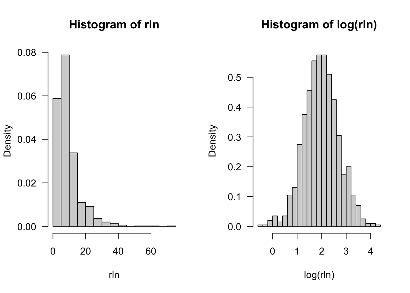
\]\(Y\) has mean \(\mu = \exp\{\alpha + \beta/2\}\) and variance \(\sigma^2 = (e^\beta - 1) \exp\{2\alpha + \beta\}\). If \(Y \sim \text{Lognormal}(\alpha,\beta)\), then \(\log Y\) has a Gaussian distribution with mean \(\alpha\) and variance \(\beta\). We can also construct a log-normal variable from a standard Gaussian: if \(Z \sim G(0,1)\), then \(Y = \exp\{\alpha + \beta Z\}\) has a log-normal distribution. Figure 28.6 shows the histogram of 1,000 random samples from a Lognormal(2,1/2) distribution and the histogram of the log-transformed values.
Figure 28.6: Histograms of 1,000 random samples from \(Y \sim \text{Lognormal}(2,1/2)\) and of \(\log Y\).
Box-Cox family
The Box-Cox family of transformations is a special case of power transformations that was introduced by Box and Cox (1964). Most commonly used is the one-parameter version of the Box-Cox transformation \[
y^{(\lambda)} = \left \{
\begin{array}{ll}
\frac{y^\lambda - 1}{\lambda} & \text{if } \lambda \ne 0 \\
\log y & \text{if } \lambda = 0
\end{array}\right.
\tag{28.1}\]
This transformation applies if \(y > 0\). For the more general case, \(y > -c\), the two-parameter Box-Cox transformation can be used \[
y^{(\lambda)} = \left \{
\begin{array}{ll}
\frac{(y+c)^\lambda - 1}{\lambda} & \text{if } \lambda \ne 0 \\
\log (y+c) & \text{if } \lambda = 0
\end{array}\right.
\]
\(c\) is simply a value by which to shift the distribution so that \(y+c > 0\). The key parameter in the Box-Cox transformation is \(\lambda\).
The term \(- 1\) in the numerator and the division by \(\lambda\) for \(\lambda \ne 0\) in Equation 28.1 are linear operations that do not affect the proximity to normality of \(y^{(\lambda)}\). An abbreviated version of Equation 28.1 is
For a given value of \(\lambda\), the transformation is monotonic, mapping large values to large values if \(\lambda > 0\) and large values to small values if \(\lambda < 0\). The transformation thus retains the ordering of observations (Figure 28.7).
Figure 28.7: Box-Cox transformations for various values of \(\lambda\)
How do we find \(\lambda\)? If the assumption is that for some value \(\widehat{\lambda}\) the distribution of \(y^{(\widehat{\lambda})}\) is Gaussian, then \(\lambda\) can be estimated by maximum likelihood assuming a Gaussian distribution–after all, we are looking for the value of \(\lambda\) for which the Gaussian likelihood of the transformed data is highest.
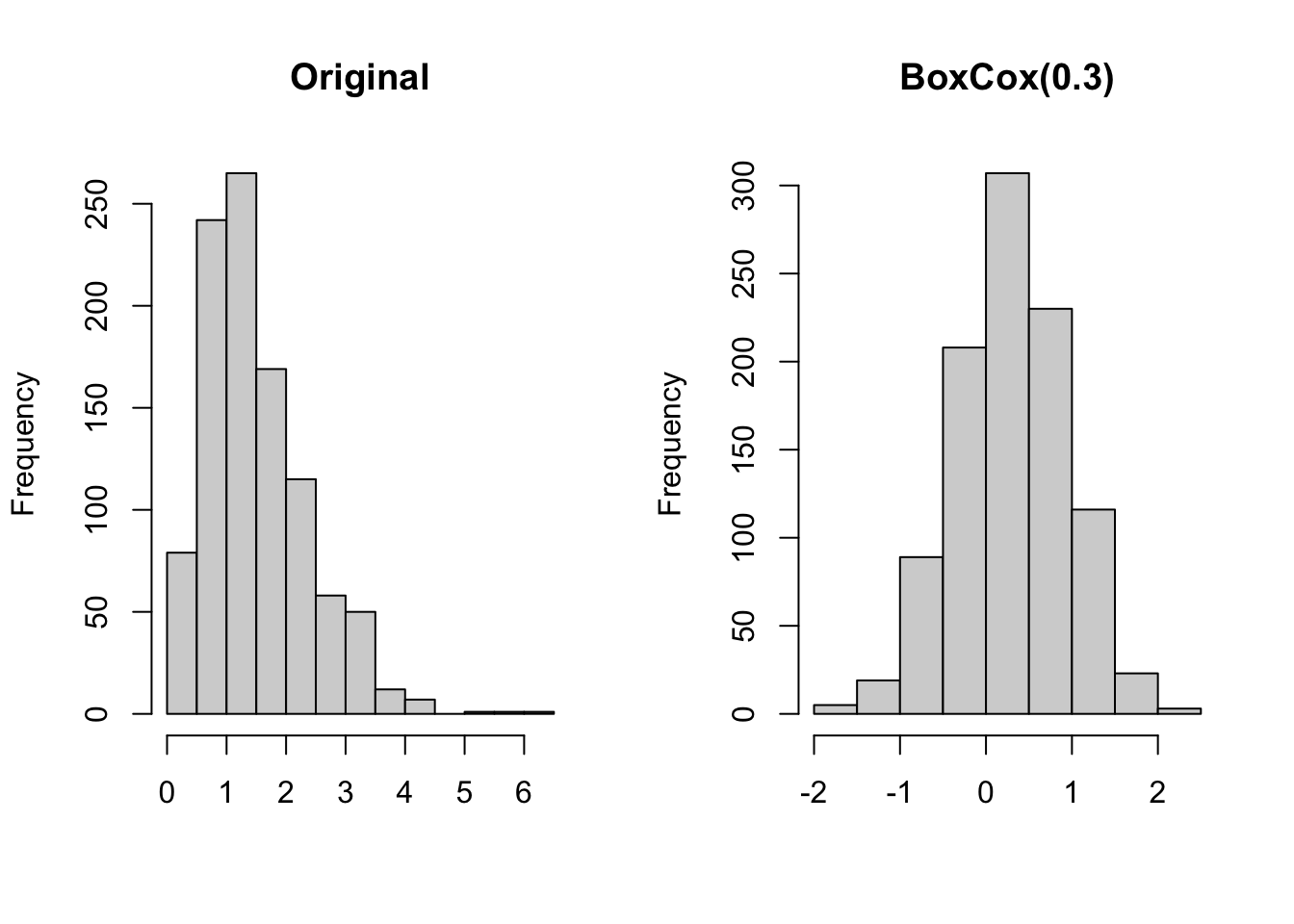
Figure 28.8: Original and Box-Cox-transformed data drawn from a Gamma(3,2) distribution.
The following Python code simulates 1,000 samples from a Gamma(3,2) distribution and from a Lognormal(2,1) distribution.
import numpy as npnp.random.seed(234)x1 = np.random.gamma(shape=3,scale=2,size=1000)x1 = np.reshape(x1,(-1,1))# numpy's lognormal distribution uses the mean and standard deviation# of the underlying normal distribution as parameters x2 = np.random.lognormal(mean=2,sigma=1,size=1000)x2 = np.reshape(x2,(-1,1))
The PowerTransformer method in sklearn.preprocessing estimates the \(\lambda\) parameter of the Box-Cox transformation. We expect the estimate for the log-normal data to be close to zero, since a log transformation (\(\lambda=0\)) of a log-normal random variable yields a Gaussian random variable.
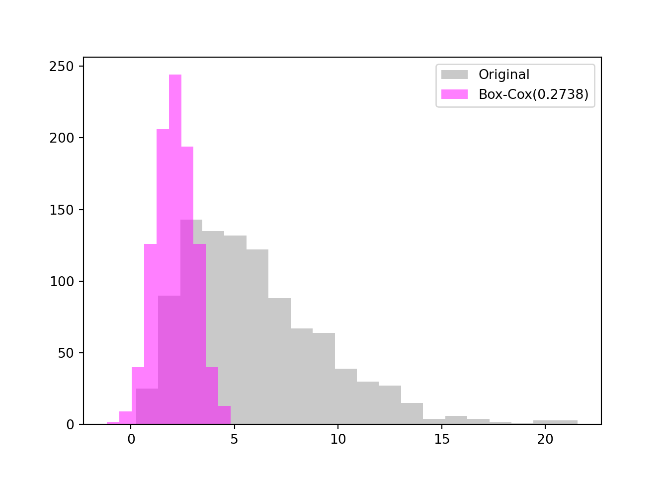
The estimate of \(\lambda\) to transform the Gamma(3,2) data is \(\widehat{\lambda} = 0.2738\) and the estimate to transform the log-normal data is \(\widehat{\lambda} = 0.0135\). The impact on the distribution of the transformed Gamma data is shown in Figure 28.9.
Figure 28.9: 1,000 samples from Gamma(3,2) and Box-Cox transformation with \(\widehat{\lambda} = 0.2738\).
Yeo-Johnson transformation
Yeo and Johnson (2000) proposed an improvement of the Box-Cox transformation to permit negative values. While the two-parameter Box-Cox transformation shown above, which introduces the lower bound parameter \(c\) allows for \(y \ge -c\), this still imposes a lower bound on the value of \(y\). The Yeo-Johnson transformation does not require a lower bound. Their power transformation is
The transformation is constructed to have a continuous second derivative at \(y = 0\), forcing a smooth transition at zero. The parameter \(\lambda\) can be estimated by maximum likelihood, as for the Box-Cox transformation.
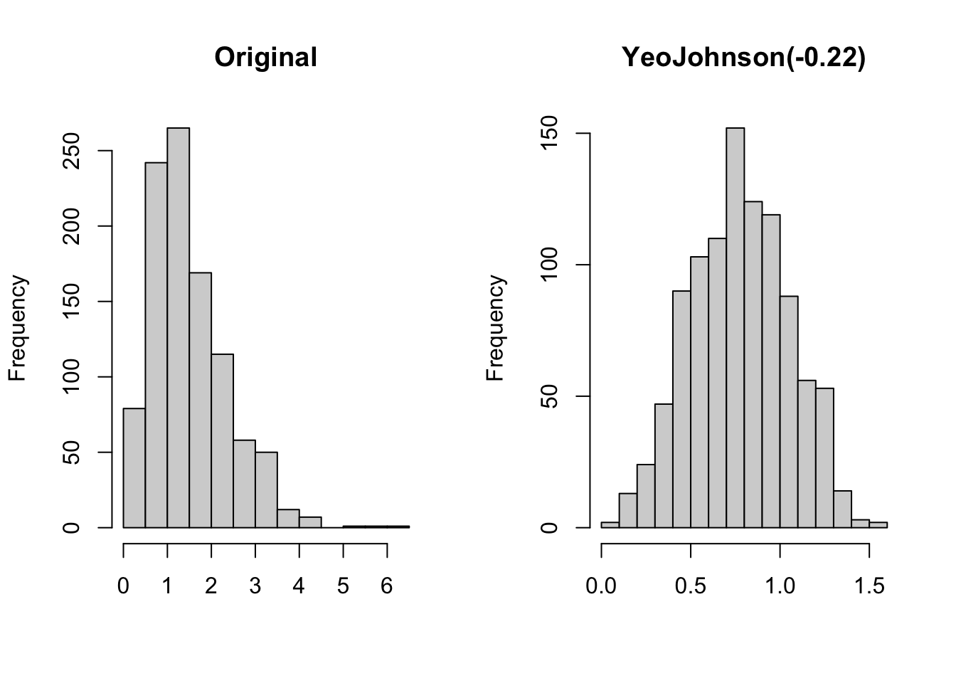
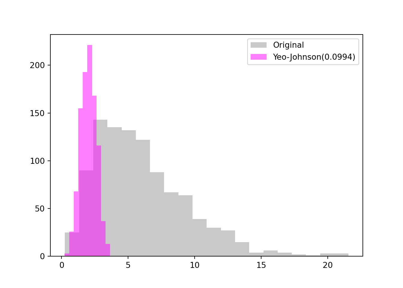
Figure 28.10: 1,000 samples from Gamma(3,2) and Yeo-Johnson transformation with \(\widehat{\lambda} = 0.0994\).
Quantile transformation
The Box-Cox transformation does a good job to transform the data closer to a Gaussian distribution in the previous examples. It is not fail safe, however. Data that appear uniform or data with multiple modes do not transform to normality easily with the Box-Cox family.
However, a transformation based on the quantiles of the observed data can achieve this. In fact, you can use quantiles to generate data from any distribution.
If \(Y\) is a random variable with c.d.f. \(F(y) = \Pr(Y \le y)\), then the quantile function \(Q(p)\) is the inverse of the cumulative distribution function; for a given probability \(p\), it returns the value \(y\) for which \(F(y) = p\).
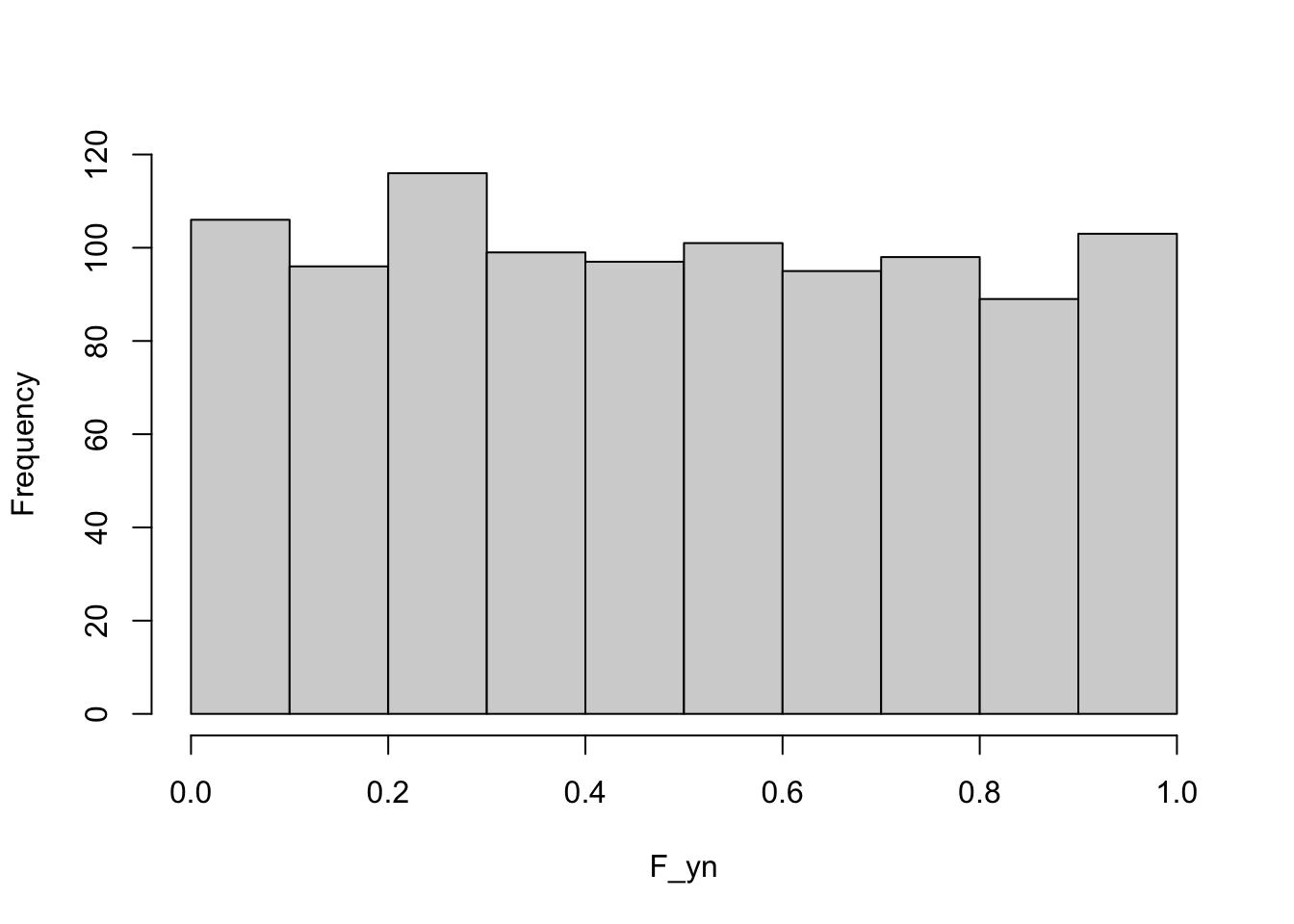
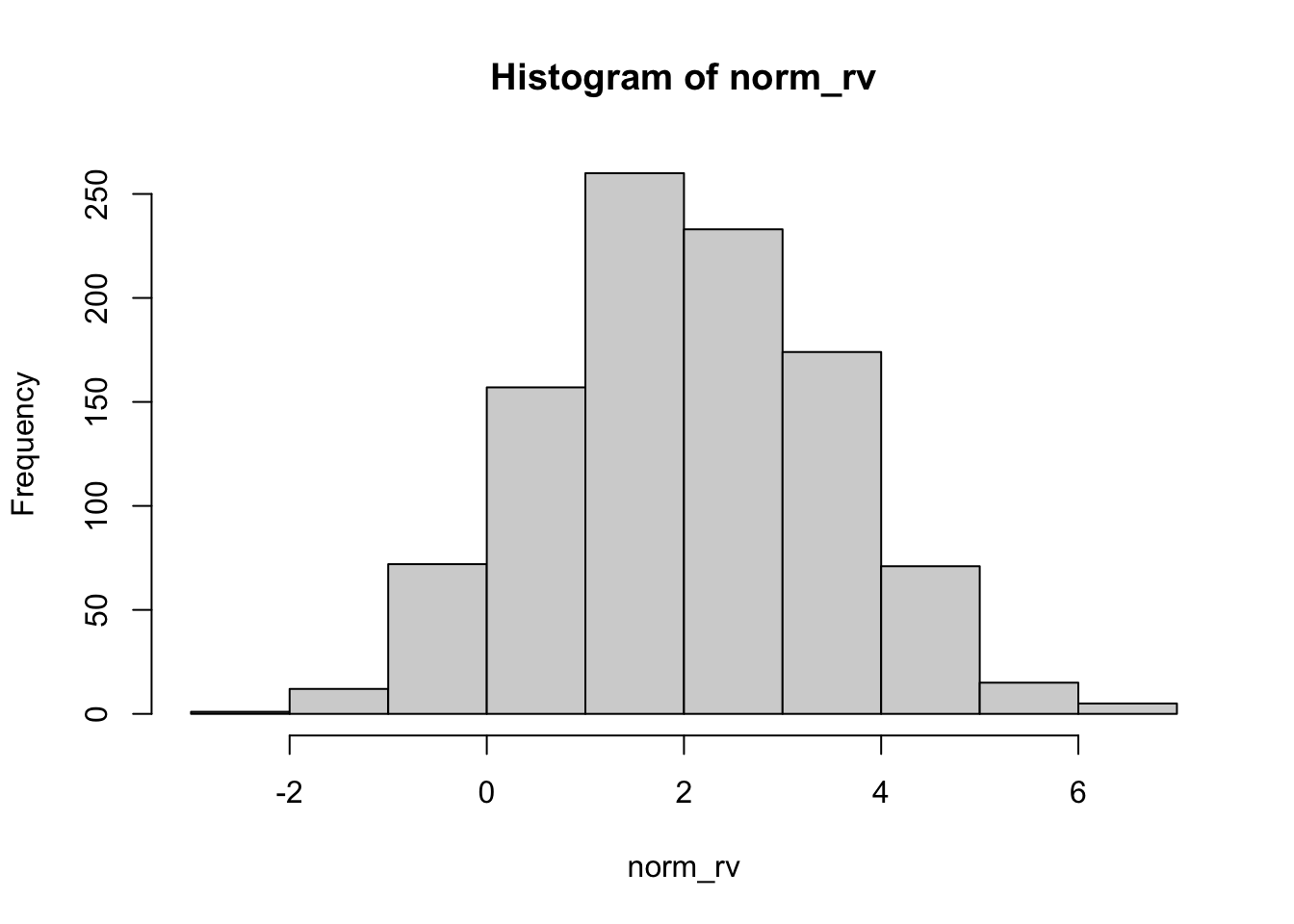
Now here is a possibly surprising result: if \(Y\) has c.d.f. \(F(y)\), then we can think of the c.d.f as a transformation of \(Y\). What would its distribution look like? The following R code draws 1,000 samples from a G(\(2,1.5^2\)) distribution and plots the histogram of the c.d.f. values \(F(y)\).
The distribution of \(F(y)\) is uniform on (0,1)—this is true for any distribution, not just the Gaussian.
We can combine this result with the following, possibly also surprising, result: If \(U\) is a uniform random variable, and \(Q(p)\) is the quantile function of \(Y\), then \(Q(u)\) has the same distribution as \(Y\). This is how you can generate random numbers from any distribution if you have a generator of uniform random numbers: plug the uniform random numbers into the quantile function.
These are the key results behind quantile transformation, mapping one distribution to another based on quantiles.
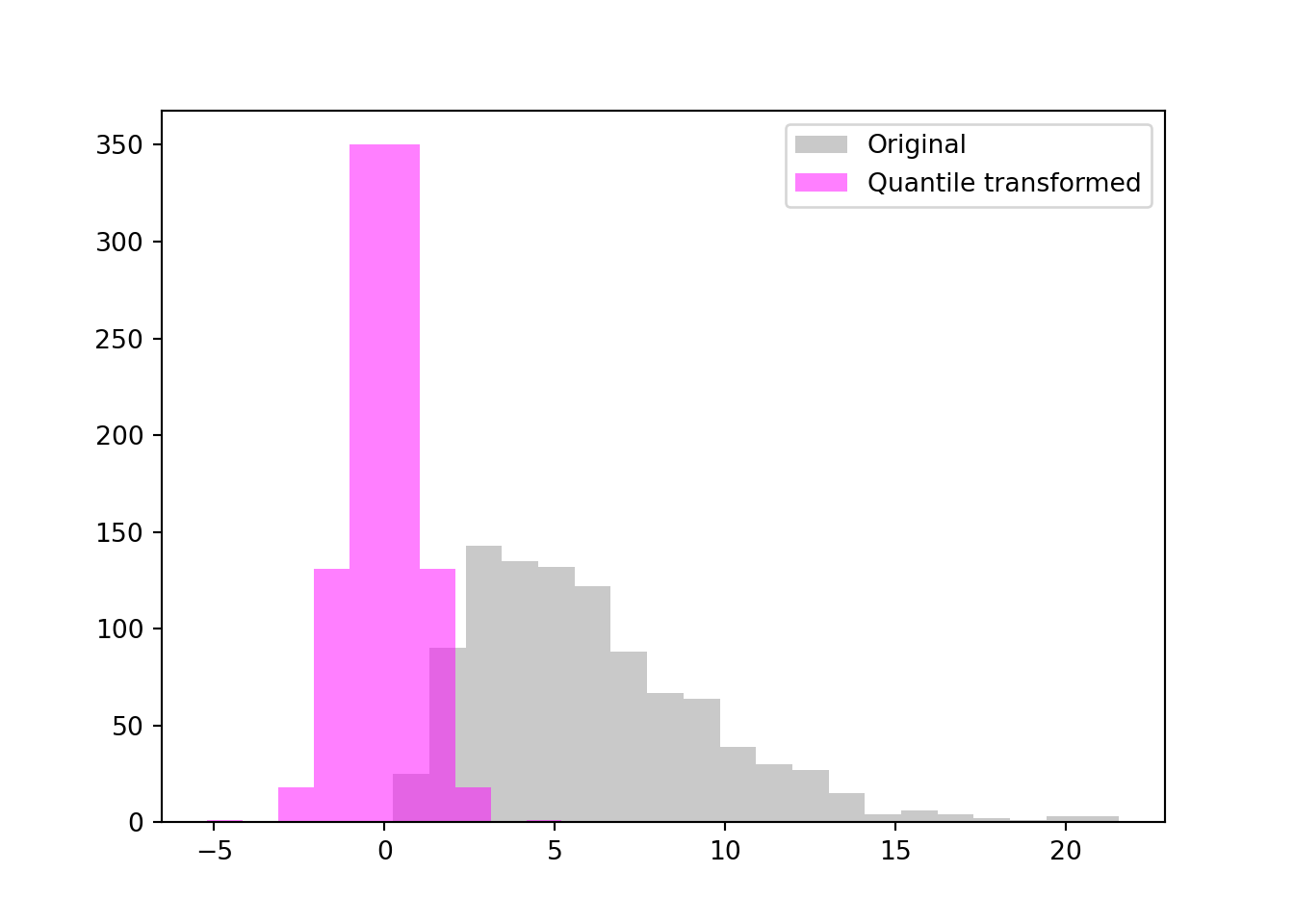
The QuantileTransformer in sklearn.preprocessing can transform data based on quantiles to a uniform (default) or a Gaussian distribution. The results of transformation to normality for the Gamma(3,2) data are shown in Figure 28.11. These are not very different from the results of the Box-Cox transformation. However, the quantile transformation method always works, even in cases where the Box-Cox family of transformation fails to get close to normality.
Figure 28.11: Quantile transformation to normality for Gamma(3,2) data.
To Transform or not to Transform
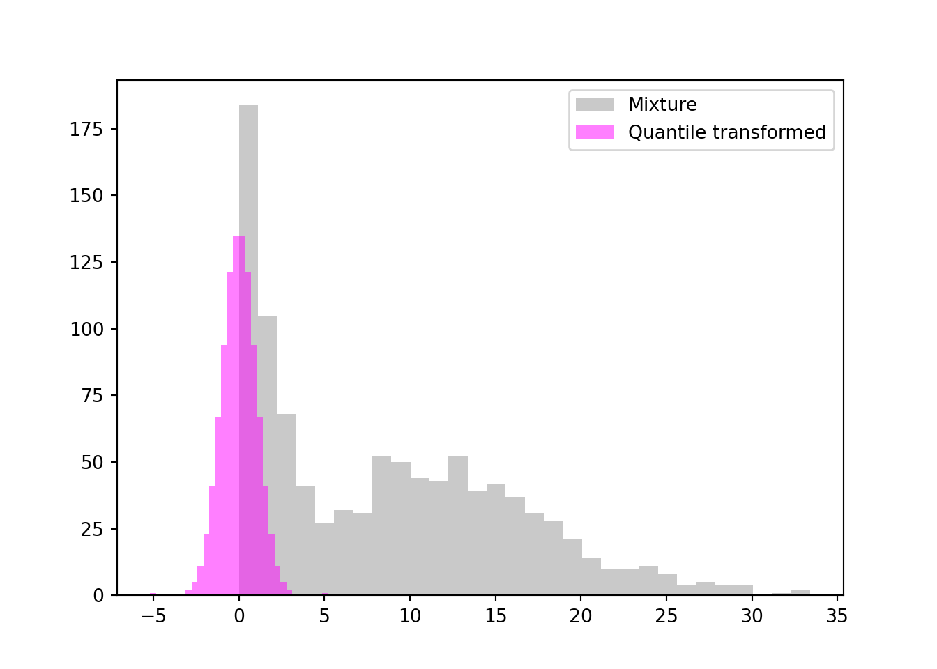
Why do we not always apply a nonlinear transform to a continuous target variable to achieve greater symmetry, stable variance, greater normality? After all, the results of the transformations are impressive. Figure 28.12 shows a quantile transformation to normality for data from a two-component mixture of Gamma densities. The bimodal distribution maps to a standard Gaussian like magic.
Figure 28.12: Quantile transformation to normality for bimodal data from a mixture distribution.
What are you giving up by analyzing the transformed target instead of the original target?
When the goal of data analytics is testing research hypotheses, we usually observe the target variable of interest and formulate hypotheses about its properties. What do these hypotheses mean in terms of the transformed data? This is not a lways clear, in particular when highly nonlinear transformations such as quantiles are involved.
The parameters of the distribution of \(Y^*\), the transformed target, are not estimating the parameters of the distribution of \(Y\). The mean of \(\log Y\) is not the log of the mean of \(Y\). When the transformation can be inverted, we usually end up with biased estimators. For example, if \(Y\) has a Lognormal(\(\alpha,\beta\)) distribution, then \(\overline{Y}\) is an unbiased estimate of \[
\text{E}[Y] = \exp\{\alpha + \beta/2\}
\]
If we log-transform the data the sample mean of the transformed data \(y^* = \log y\) estimates \[
\text{E}[\overline{Y}^*] = \frac{1}{n}\sum_{i=1}^n \text{E}[\log Y_i]
\] The exponentiation of this estimator is not an unbiased estimator of \(\text{E}[Y]\).
Box, G. E. P., and D. R. Cox. 1964. “An Analysis of Transformations.”Journal of the Royal Statistical Society. Series B (Methodological) 26 (2): 211–52. http://www.jstor.org/stable/2984418.
Yeo, In‐Kwon, and Richard A. Johnson. 2000. “A new family of power transformations to improve normality or symmetry.”Biometrika 87 (4): 954–59. https://doi.org/10.1093/biomet/87.4.954.