17 Introduction

Quotes

It would be nice if we could just plug data into a statistical model,
crunch the numbers, and take for granted that it was a good
representation of the real world.
Nate Silver, The Signal and the Noise

Modeling data is a key activity for data scientists. Here we apply computational thinking to create a solution to a data science problem by training algorithms on data. The result is a model that describes the training data sufficiently well so that it generalizes to new observations. When presented with new data the model can be used to predict, forecast, classify, cluster, associate, or recommend an outcome or course of action.

Modeling data is such an important activity in data science projects that it is often thought of as the most important activity or even the only thing that matters. Because there are many modeling alternatives to choose from, because they need to be understood from a theoretical as well as a practical perspective, because building a great versus a sub-optimal model can make or break a project, data science education spends much time on data modeling.

The material presented here is foundational and we cannot dive deep into all aspects of modeling data. The goal of this module is to provide an introduction and to set the stage for more in-depth coverage later on by conveying essential concepts such as data-based learning approaches, the bias-variance tradeoff, the testing and validation of models, and the establishment of causation.

Recall that all models obey the same simple structure: an input is processed by some algorithm into some form of output (Figure 3.4). In Figure 3.5 an attempt was made to structure the input, algorithm, and output components. Depending on the type of output, for example, prediction, classification, or clustering, and depending on the type of input (structured or unstructured data, for example), we have choices on how to train a model.

The data scientist’s task is to understand the possible choices, select a reasonable class of models, and train the model algorithm appropriately to achieve the goals of the project. Wait, what? Is training not simple and automatic? Not at all. Using the same set of data, even the same software, chances are that data scientists will train their models differently. Decisions need to be made about parameters of the training algorithm that affect the determination of parameters of the model itself. For example, choosing a learning rate parameter can affect the values a training algorithm determines as optimal. Modeling data is an art and a science.

17.1 Statistical Models

The models you train in data science applications are statistical models, they are trained on data that is inherently uncertain. Sources of uncertainty might be the random sampling of observations from a population, the random assignment of treatments to experimental units, measurement variability, natural variability of an attribute, incompleteness of the models, and so on.

Statistical models are a subset of mathematical models. A mathematical model abstracts a concrete system using mathematical concepts. For example, we can model mathematically how much space is in a box, the trajectory a baseball will travel, or how closely we can package items on a shelf. While a mathematical model describes a system in deterministic terms, statistical models are non-deterministic, they allow for the presence of uncertainty.

The non-determinism of statistical models is a feature and a strength. The random elements of the model allow us to develop models that are simpler (more parsimonious) than equivalent mathematical models that must capture the salient features deterministically. Randomness is an antidote to complexity as long as the random elements can be described through their distributional properties. It does come at a cost, however.

Statistical models are a subset of mathematical models, and they also belong to the class of stochastic models. A stochastic model describes the probability distribution of outcomes by allowing one or more of the model elements to be random variables. Like stochastic models, statistical models use random variables and their probability models to capture the effects of random processes. Like mathematical models, statistical models involve mathematical relationships that are governed by parameters; unknown constants that are determined based on training data.

Definition: Statistical Model

A statistical model is a stochastic model that contains random variables and unknown constants. The unknown constants are called parameters and are estimated based on data. Parameters are constants, not random variables. The estimator of a parameter that depends on data is a random variable since the data are random.

Example: Modeling Coin Flips

Suppose that you want to develop a model that can predict whether a coin lands on heads or tails. A deterministic mathematical model would capture the physics of the coin itself, the medium through which it travels, and the surface on which it lands. It would take into account the shape of the coin and the condition of its surface. It would account for direction and strength of air movement, the angle and force with which the coin is released, and so on. The model would be very complex. If the various forces and variables that affect the coin—as well as their interactions—are captured correctly, the model could be very accurate. However, change an element of the process, for example, make the coin travel through moist air rather than dry air or land on grass, and you would have to revisit the model.

A much simpler model is one that describes the coin behavior in a probabilistic (non-deterministic) way. The various forces affecting whether the coin lands on heads or tails are essentially random affects that balance each other out. The end result is the following: if the coin is fair (balanced), it will land on heads or tails with equal probability. This model is extremely simple, it has no parameters. The behavior of the coin is described not in terms of what happens in any one coin toss, but in terms of the distribution of results that is realized when the random effects play out: the coin toss is modeled as a Bernoulli (binary) distribution with an event probability of 0.5. On aveage you will observe as many coins landing on heads and tails, but you cannot say for sure what the outcome of the next coin toss will be. We have to guess it. That guess is a prediction under the model. Since the outcome itself is uncertain, the prediction carries with it also some uncertainty. If the coin is tossed twenty times we would predict 10 heads and 10 tails and would not be surprised if 9 heads or 11 heads turned up.

If there are doubts whether the coin in question is fair, we can run a little experiment. Flip the coin a hundred times and observe the number of heads (or tails) that appear. If we see 65 out of 100 heads, we’ll model the distribution of coin flips as a Bernoulli distribution with an event probability of 0.65.

What did we gain and what did we give up in the coin flip example by using a probabilistic formulation instead of a deterministic model? We gained a much simpler model that is easily understood and is very general. It applies to pretty much all coin flips, regardless of the conditions. It is a very parsimonious model that depends on just one parameter: the probability that heads (or tails) will turn up. And we have a simple recipe to estimate that parameter if we need to.

We lost, however, the ability to determine the outcome of any one coin toss. We cannot say with certainty whether a coin toss results in heads or tails. We can only state how likely the outcome will be. By incorporating uncertainty (randomness) in the model we made the model simpler but we transferred uncertainty into the model output. In data science applications we are just fine with that. Because our input material—data—is inherently uncertain we cannot expect to produce deterministic models. Quantifying the uncertainty in the model outputs is an important part of modeling data with statistical approaches.

The process of training a statistical model to a set of data is called statistical learning. Here is a more precise definition:

Definition: Statistical Learning

Statistical Learning is the process of understanding data through the application of tools that describe structure and relationships in data. Models are formulated based on the structure of data to predict or classify outcomes from inputs, to test hypothesis about relationships, to group data, to find association, to reduce the dimensionality of a problem, and so on.

If data science is concerned with statistical models and uses statistical learning to understand the structure and relationships in data, then what about machine learning models? Do they fall outside of data science?

Statistical Learning and Machine Learning

Much is being made of the difference between statistical models and machine learning models, or to be more precise, between statistical learning (SL) and machine learning (ML).

Statistical learning emphasizes prediction more than the testing of hypothesis, as compared to classical statistical modeling. Many model classes used in statistical learning are the same models one uses to test hypothesis about patterns and relationships in data. Emphasis of prediction over hypothesis testing—or vice versa—flows from the nature of the problem we are trying to solve. The same model can be developed with focus on predictive capability or with focus on interpretability. We do not want to overdo the distinction between statistical learning and statistical modeling: statistical learning uses statistical models.

Learning is the process of converting experience into knowledge and machine learning is an automated way of learning by using computers and algorithms. Rather than directly programming computers to perform a task, machine learning is used when the tasks are not easily described and communicated (e.g., driving, reading, image recognition) or when the tasks exceed human capabilities (e.g., analyzing large and complex data sets). Modern machine learning discovered data as a resource for learning and that is where statistical learning and machine learning meet.

SL and ML have more in common, than what separates them:

The input to a learning algorithm is data; the raw material is the same.
The data are thought of as randomly generated, there is some sense of variability in the data that is attributed to random sources.
Both disciplines distinguish supervised and unsupervised forms of learning
They use many of the same models and algorithms for regression, classification, clustering, dimension reduction, etc.

Machine learning uses observed data to describe relationships and “causes”; the emphasis is on predicting new and/or future outcomes. There is comparatively little emphasis on experimentation and hypothesis testing.

A key difference between SL and ML is what Breiman (2001) describes as the difference between data modeling and algorithmic modeling and aligns closely with statistical and machine learning thinking. In data modeling, theory focuses on the probabilistic properties of the model and of quantities derived from it. In algorithmic modeling, the focus is on the properties of the algorithm itself: starting values, optimization, convergence behavior, parallelization, hyperparameter tuning, and so on. Consequently, statisticians are concerned with the asymptotic distributional behavior of estimators and methods as $n \rightarrow \infty$. Machine learning focuses on finite sample properties and asks what accuracy can be expected based on the available data.

The strong assumptions statisticians make about the stochastic data-generating mechanism that produced the data set in hand are not found in machine learning. That does not mean that machine learning models are free of stochastic elements and assumptions—quite the contrary. It means that statisticians use the data-generating mechanism as the foundation for conclusions rather than the data alone.

When you look at a p-value in a table of parameter estimates, you rely on all assumptions about distributional properties of the data, correctness of the model, and (asymptotic) distributional behavior of the estimator. These flow explicitly from the data-generating mechanism or implicitly from somewhere else. Otherwise, the p-value does not make much sense. (Many argue that p-values are not very helpful to begin with and possibly even damaging to decision making but this is not the point of the discussion here.)

If you express the relationship between a target variable $Y$ and inputs $x_1, \cdots, x_p$ as

\[ Y = f(x_1,\cdots,x_p) + \epsilon \]

where $\epsilon$ is a random variable, it does not matter whether you perform data modeling or algorithmic modeling. We need to think about $\epsilon$ and its properties. How does $\epsilon$ affect the algorithm, the prediction accuracy, the uncertainty of statements about $Y$ or $f(x_1, \cdots, x_p)$? That is why all data professionals need to understand about stochastic models and statistical models.

17.2 Example: Logistic Regression Model

Suppose we are charged with developing a model to predict recurrence of cancer. There are many possible aspects that influence the outcome. These are potential input variables to our model:

Age, gender
Medical history
Lifestyle factors (nutrition, exercise, smoking, …)
Type of cancer
Size of the largest tumor
Site of the cancer
Time since diagnostic, time from treatment
Type of treatment
and so on

If we were to try and build a deterministic model that predicts cancer recurrence perfectly, all influences would have to be taken into account and their impact on the outcome would have to be incorporated correctly. That would be an incredibly complex—and impractical—model.

By taking a stochastic approach we acknowledge that there are processes that affect the variability in cancer recurrence we observe from patient to patient. The modeling can now focus on the most important factors and how they drive cancer recurrence. The other factors are included through random effects. If the model captures the salient factors and their impact correctly, and the variability contributed by other factors is not too large, and not systematic, the model is very useful. It possibly is much more useful than an inscrutably complex model that tries to accommodate all influences perfectly.

The simplest stochastic model for cancer recurrence is to assume that the outcome is a Bernoulli (binary) random variable taking on two states (cancer recurs, cancer does not recur) with probabilities $\pi$ and $1-\pi$. If we code the two states numerically, cancer recurs as 1, cancer does not recur as 0, the probability mass function of cancer recurrence is that of the random variable $Y$,

\[ \Pr(Y=y) = \left \{ \begin{array}{cl} \pi & y=1 \\ 1-\pi & y = 0\end{array} \right . \]

The parameter in our cancer model is $\pi$, the probability that $Y$ takes on the value 1. Unlike the coin flip example earlier in the chapter, we do not know $\pi$ and must estimate it from data. And $\pi$ will not be a single number. The probability of cancer recurrence will be a function of some or all of the input variables.

Success and Failure

In statistics, the probability $\pi$ for the event coded as $Y=1$ is frequently called the “success” probability and its complement is called the “failure” probability. We prefer to call them the “event” and “non-event” probabilities instead to avoid the awkward situation to label cancer recurrence a “success”. The event is the binary outcome coded as a 1.

Because we cannot visit with all cancer patients, a sample of patients is used to estimate $\pi$. This process introduces uncertainty into the estimator of $\pi$, a larger sample will lead to a more precise (a less uncertain) estimator.

The model is overly simplistic in that it captures all possible effects on cancer recurrence in the single quantity $\pi$. Regardless of age, gender, type of cancer, etc., we would predict a randomly chosen cancer patient’s likelihood to experience a recurrence as $\pi$. To incorporate input variables that affect the rate of recurrence we need to add structure to $\pi$. A common approach in statistical learning and in machine learning is that inputs have a linear effect on a transformation of the probability $\pi$:

\[ g(\pi) = \beta_0 + \beta_1 x_1+\cdots + \beta_p x_p \tag{17.1}\]

The interpretation of Equation 17.1 is that the effects of the inputs manifest in an additive fashion, each input is scaled by a coefficient $\beta$. But the effects do not act additively (linearly) on the event probability. They act additively on a transformation of the event probability.

When $g(\pi)$ is the logit function

\[\log\left \{ \frac{\pi}{1-\pi} \right\}\]

the model is called a logistic regression model. $x_1,\cdots,x_p$ are the inputs of the model, $\beta_0, \cdots, \beta_p$ are the parameters of the model.

If we accept that the basic structure of the logistic model applies to the problem of predicting cancer occurrence, we use our sample of patient data to

estimate the parameters $\beta_0, \cdots, \beta_p$;
determine which inputs and how many inputs are adequate: we need to determine $p$ and the specific input variables;
determine whether the logit function is the appropriate transformation that achieves linearity of the input effects.

The effect of the inputs is called linear on $g(\pi)$ if $g(\pi)$ is a linear function of the parameters. To test whether this is the case take derivatives of the function with respect to all parameters. If the derivatives do not depend on parameters, the effect is linear.

\[ \begin{align*} \frac{\partial g(\pi)}{\partial\beta_{0}} &= 1 \\ \frac{\partial g(\pi)}{\partial\beta_{1}} &= x_{1}\\ \frac{\partial g(\pi)}{\partial\beta_{p}} &= x_{p} \\ \end{align*} \]

None of the derivatives depends on any of the $(\beta_{0},\ldots,\beta_{p})$. We conclude that $g(\pi)$ is linear in the parameters. A non-linear function is non-linear in at least one parameter.

Example: Plateau (hockey stick) Model

A plateau model reaches a certain amount of output and remains flat afterwards. When the model prior to the plateau is a simple linear model, the plateau model is also called a hockey-stick model.

The point at which the plateau is reached is called a change point. Suppose the change point is denoted $\alpha$. The hockey-stick model can be written as

\[ \text{E} \lbrack Y\rbrack = \left\{ \begin{matrix} \beta_{0} + \beta_{1}x & x \leq \alpha \\ \beta_{0} + \beta_{1}\alpha & x > \alpha \end{matrix} \right. \]

If $\alpha$ is an unknown parameter, this is a non-linear model.

17.3 Model Components

A statistical model has random elements, expressed through the distribution of random variables in the model and systematic components that describe the mathematical relationship between inputs and target variables. Another way of phrasing this: a statistical model contains noise and signal(s). The task of modeling data is to figure out which is which.

The expression for the logistic regression model

\[ g(\pi) = \beta_{0} + \beta_{1}x_{1} + \ldots + \beta_{p}x_{p} \]

looks quite different from the model introduced earlier,

\[ Y = f\left( x_{1},\ldots,x_{p} \right) + \epsilon \]

Where is the connection?

The error term $\epsilon$ is a random variable and we need to specify some of its distributional properties to make progress. At a minimum we provide the mean and variance of $\epsilon$. If the model is correct—correct on average—then the error terms should have a mean of zero and not depend on any input variables (whether those in the model or other inputs). A common assumption is that the variance of the errors is a constant and not a function of other effects (fixed or random). The two assumptions are summarized as $\epsilon \sim \left( 0,\sigma^{2} \right)$; read as $\epsilon$ follows a distribution with mean 0 and variance $\sigma^{2}$.

Mean Function

Now we can take the expected value of the model and find that

\[ \text{E}\lbrack Y\rbrack = \text{E}\left\lbrack f\left( x_{1},\ldots,x_{p} \right) + \epsilon \right\rbrack = f\left( x_{1},\ldots,x_{p} \right) + \text{E}\lbrack\epsilon\rbrack = f\left( x_{1},\ldots,x_{p} \right) \]

Because the errors have zero mean and because the function $f\left( x_{1},\ldots,x_{p} \right)$ does not contain random variables, $f\left( x_{1},\ldots,x_{p} \right)$ is the expected value (mean) of $Y$. $f\left( x_{1},\ldots,x_{p} \right)$ is thus called mean function of the model.

Example: Curvilinear Models

Polynomial models such as a quadratic model \[ Y = \beta_{0} + \beta_{1}x + \beta_{2}x^{2} + \epsilon \] or cubic model \[ Y = \beta_{0} + \beta_{1}x + \beta_{2}x^{2} + \beta_{3}x^{3} + \epsilon \] have a curved appearance when $Y$ is plotted against $x$. They are linear models in the parameters and they are non-linear models in the $x$s.

To test this, take derivatives of the mean function with respect to the parameters. For the quadratic model the partial derivatives with respect to $\beta_{0}$, $\beta_{1}$, and $\beta_{2}$ are 1, $x$, and $x^{2}$, respectively. The model is linear in the parameters.

To emphasize that the models are not just straight lines in $x$, a linear model with curved appearance is called curvilinear.

What does the mean function look like in the logistic regression model? The underlying random variable $Y$ has a Bernoulli distribution. Its mean is

\[ \text{E}\lbrack Y\rbrack = \sum y\, \Pr(Y = y) = 1 \times \pi + 0 \times (1 - \pi) = \pi \]

The logit function \[ g(\pi) = \log \left\{ \frac{\pi}{(1 - \pi)} \right\} \] is invertible and the model \[ g(\pi) = \beta_0 + \beta_1 x_{1} + \ldots + \beta_p x_p \]

can be written as

\[ \text{E}\lbrack Y\rbrack = \pi = g^{- 1}\left( \beta_{0} + \beta_{1}x_{1} + \ldots + \beta_{p}x_{p} \right) \]

The mean function of the logistic model is also a function of the inputs.

Exercise

Show that if $g(\pi)$ is the logit function, the mean function can be written as

\[ \pi = \frac{1}{1 + \text{E}\left\{ - \beta_0 - \beta_1 x_1 - \cdots - \beta_p x_p \right\}} \] Show that although $g(\pi)$ is linear in the parameters, $\pi$ is a non-linear function of the parameters.

Systematic Component

The mean functions \[ f\left( x_{1},\ldots,x_{p} \right) \] and \[\frac{1}{1 + \text{E}\left\{ - \beta_{0} - \beta_{1}x_{1} - \ldots - \beta_p x_p \right\} } \] look rather different, except for the input variables $x_{1},\ldots,x_{p}$.

With the model $Y = f\left( x_{1},\ldots,x_{p} \right) + \epsilon$ we did not specify how exactly the mean function depends on parameters. There are three general approaches.

Linear predictors

The systematic component has the form of a linear predictor, that is, a linear combination of the inputs. The linear predictor is frequently denoted as $\eta$: \[ \eta = \beta_{0} + \beta_1 x_1 + \cdots + \beta_p x_p \]

The parameter $\beta_0$ is called the intercept of the linear predictor. Although optional, it is included in most models to capture the effect on the mean if no input variables are present. Models with a linear predictor and an intercept have $p + 1$ parameters in the mean function. The interpretation of $\beta_0$ is simply as the value of $\eta$ when all $x$s are 0: $x_1 = x_2 = \cdots = x_p =0$. This might be an impossible configuration. Even so, we usually leave the intercept in the model; if the $x$s can be zero simultaneously, we would not necessarily predict $\eta = 0$.

The logistic regression model in Section 17.2 also contains a linear predictor. Depending on whether you write the model in terms of $\pi$ or $g(\pi)$, the expressions are

\[ \begin{align*} g(\pi) &= \eta \\ \pi &= \frac{1}{1 + \text{E}\{ - \eta \}}\\ \end{align*} \]

Non-linear functions

The mean function can be a general non-linear function of the parameters. The number of input variables and the number of parameters can be quite different.

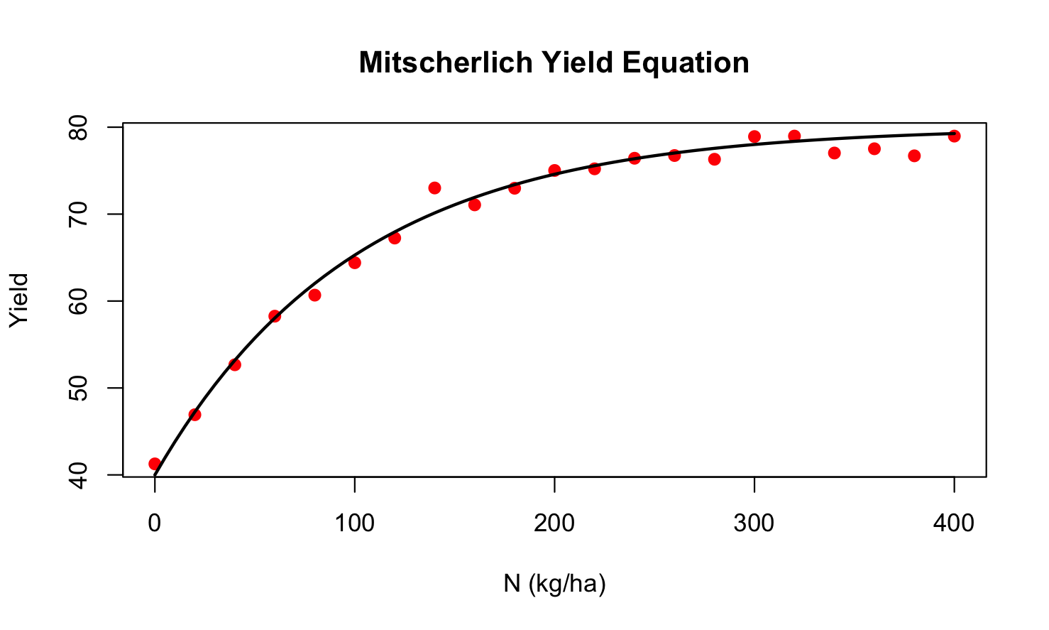
Example: Mitscherlich Model

The Mitscherlich model is popular in agricultural studies to model plant growth as a function of an input such as a fertilizer. If $Y$ denotes plant yield and $x$ denotes the amount of input, the Mitscherlich model is

\[ Y = f(x,\xi,\lambda,\kappa) + \epsilon = \lambda + (\xi - \lambda)\text{E}\left\{ - \kappa x \right\} + \epsilon \]

The mean function $f$() depends on one input variable $x$ and three parameters $(\xi,\lambda,\kappa)$. Taking derivatives, it is easily established that the mean function is non-linear (in the parameters):

\[ \frac{\partial f(x,\xi,\lambda,\kappa)}{\partial\xi} = \text{E}\{ - \kappa x \} \]

The derivative with respect to $\xi$ depends on the $\kappa$ parameter.

Non-linear equations like the Mitscherlich model are appealing because they are easily interpretable. The parameters have meaning in terms of the subject domain:

$\xi$ is the crop yield if no fertilizer is applied, the mean of $Y$ at $x = 0$. This is the baseline yield.
$\lambda$ is the upper yield asymptote as $x$ increases.
$\kappa$ relates to a rate of change, how quickly the yield increases from $\xi$ and reaches $\kappa$.

Figure 17.1 shows the Mitscherlich model fitted to a set of plant yield data, the input variable is the nitrogen rate applied (in kg/ha). Visual estimates for the baseline yield and the asymptotic yield are $\widehat{\xi} = 40$ and $\widehat{\lambda} = 80$.

Interpretability of the parameters allows us to answer research questions in terms of model parameters:

Is the asymptotic yield greater than 75? This can be answered with a confidence interval for the estimate of $\lambda$. If the confidence interval includes 75 the hypothesis $H: \text{Yield } > 75$ is rejected.
At what level of $x$ does yield achieve 75% of the maximum? This is an inverse prediction problem. Set yield to 75% of $\lambda$ and solve the model for $x$.
The rate of change in yield is less than ½ unit once $x = 100$ are applied. This can be answered with a hypothesis test for $\kappa$.

Smooth functions and local models

The third method of specifying the systematic component is to not write it as a function of inputs and parameters. This is common for non-parametric methods such as kernel regression models, regression splines, smoothing splines, and generalized additive models. These models still have parameters, but the relationship between inputs and parameters is implied through the method of training the models.

For example, LOESS is a local polynomial regression method. A LOESS model of degree 2 fits a quadratic polynomial model to a portion of the data (a window). The window is created by centering a weight function at the location where you want to predict; call this value $x_0$. Data points close to $x_0$ receive more weight in the analysis than data points far from $x_0$. The model at $x_0$ is the following:

\[ Y(x_0) = \beta_{00} + \beta_{10}x_0 + \beta_{20}x_0^{2} + \epsilon \]

$\beta_{00}$ is the intercept of the quadratic model fit at location $x_0$, $\beta_{10}$ is the slope with respect to $x$ at location $x_0$, $\beta_{20}$ is the slope of the quadratic term $x^2$ at location $x_0$.

To predict at a different location, $x_j$, say, the weight function is moved to $x_j$ and the local quadratic model $$ Y(x_j) = {0j} + {1j}x_j + _{2j}x_j^{2} +

$$ is fit again.

A LOESS model cannot be written as a single model with a single set of parameters. A different set of parameters applies to each prediction location $x_j$. The underlying model in each window is a known parametric model, however: a quadratic polynomial in this example.

Random Component

The random components of a statistical model are the stochastic elements that describe the distribution of the target variable $Y$. By now we are convinced that most data we work with are to some degree the result of random processes and that incorporating randomness into models makes sense. The model does not need to be correct for every observation, but it needs to be correct on average—an additive zero-mean random error is OK. Even if all influences on the output $Y$ were known, it might be impossible to measure them, or to include them correctly into the model.

Randomness is often introduced deliberately by sampling observations from a population or by randomly assigning treatments to experimental units. Finally, stochastic models are often simpler and easier to explain than other models. Among competing explanations, the simpler one wins (Occam’s Razor).

We encountered two basic approaches to reflect randomness in a statistical model:

Adding an additive error term to a mean function
Describing the distribution of the target variable

The Mitscherlich model is an example of the first type of specification:

\[ Y = f(x,\xi,\lambda,\kappa) + \epsilon = \lambda + (\xi - \lambda)\text{E}\left\{ - \kappa x \right\} + \epsilon \]

Under the assumption that $\epsilon \sim \left( 0,\sigma^{2} \right)$, it follows that $Y$ is randomly distributed with mean $f(x,\xi,\lambda,\kappa)$ and variance $\sigma^{2}$; $Y \sim \left( f(x,\xi,\lambda,\kappa),\sigma^{2} \right)$. If the model errors were normally distributed, $\epsilon \sim N\left( 0,\sigma^{2} \right)$, then $Y$ would also be normally distributed. Randomness is contagious.

The logistic regression model is an example of the second type of specification:

\[ g\left( \text{E} \lbrack Y\rbrack \right) = \beta_{0} + \beta_{1}x_{1} + \ldots + \beta_{p}x_{p} \]

and $Y$ follows a Bernoulli distribution.

It does not make sense to write the model with an additive error term unless the target variable is continuous.

Models can have more than one random element. In the cancer recurrence example, suppose we want to explicitly associate a random effect with each patient: $b_{i} \sim \left( 0,\sigma_{b}^{2} \right)$. The modified model is now

\[ g\left( \pi\ |\ b_{i} \right) = \beta_{0} + b_{i} + \ \beta_{1}x_{1} + \ldots + \beta_{p}x_{p} \]

Conditional on the patient-specific value of $b_{i}$, the model is still a logistic model with intercept $\beta_{0} + b_{i}$. Because the parameters $\beta_{0}, \cdots,\beta_{p}$ are constants (not random variables), they are referred to as fixed effects. Models that contain both random and fixed effects are called mixed models.

Mixed models occur naturally when the sampling process is hierarchical.

For example, you select apples on trees in an orchard to study the growth of apples over time. You select at random 10 trees in the orchard and chose 25 apples at random on each tree. The apple diameters are then measured in two-week intervals. To represent this data structure, we need a few subscripts.

Let $Y_{ijk}$ denote the apple diameter at the $k$^th measurement of the $j$^th apple from the $i$^th tree. A possible decomposition of the variability of the $Y_{ijk}$ could be \[ Y_{ijk} = \beta_{0} + a_{i} + \eta_{ijk} + \epsilon_{ijk} \]

where $\beta_{0}$ is an overall (fixed) intercept, $a_{i} \sim ( 0,\sigma_{a}^{2})$ is a random tree effect, $\eta_{ijk}$ is an effect specific to apple and measurement time, and $\epsilon_{ijk} \sim ( 0,\sigma_{\epsilon}^{2})$ are the model errors.

This is a mixed model because we have multiple random effects ($a_{i}$ and $\epsilon_{ijk}$). In addition, we need to decide how to parameterize $\eta_{ijk}$. Suppose that a simple linear regression trend is reasonable for each apple over time. Estimating a separate slope and intercept for each of the 10 x 25 apples would result in a model with over 500 parameters. A more parsimonious parameterization is to assume that the apples share a tree-specific (fixed) intercept and slope and to model the apple-specific deviations from the tree-specific trends with random variables:

\[ \eta_{ijk} = \left( \beta_{0i} + b_{0ij} \right) + {(\beta}_{1i} + b_{1ij})t_{ijk} \]

$t_{ijk}$ is the time that a given apple on a tree is measured. The apple-specific intercept offsets from the tree-specific intercepts $\beta_{0i}$ are model as random variables $b_{0ij} \sim ( 0,\sigma_{b_{0}}^{2})$. Similarly, $b_{1ij} \sim ( 0,\sigma_{b_{1}}^{2} )$ models the apple-specific offset for the slopes as random variables. Putting everything together we obtain

\[ Y_{ijk} = \beta_{0} + \left( \beta_{0i} + b_{0ij} \right) + {(\beta}_{1i} + b_{1ij})t_{ijk} + \epsilon_{ijk} \]

Note that $a_{i}$ was no longer necessary in this model, that role is now played by $\beta_{0i}$.

The total number of parameters in this model is 24 (1 overall intercept, 10 tree-specific intercepts, 10 tree-specific slopes, and 3 variances ($\sigma_{\epsilon}^{2}, \sigma_{b_{0}}^{2}$, $\sigma_{b_{1}}^{2}$).

This is a relatively complex model and included here only to show how the sampling design can be incorporated into the model formulation to achieve interpretable and parsimonious models and how this naturally leads to multiple random effects.

A further refinement of this model is to recognize that the measurements over time for each apple are likely not independent. Furthermore, diameter measurements on the same apple close in time are more strongly correlated than measurements further apart. Incorporating this correlation structure into the models leads to a mixed model with correlated errors.

Response (Target) Variable

A model has inputs that are processed by an algorithm to produce an output. When the output is a variable to be predicted, classified, or grouped, we refer to it with different—but interchangeable—names as the response variable, or the target variable, the output or the dependent variable. We are not very particular =about what you call the variable, as long as we agree on what we are talking about—the left-hand side of the model.

Dependent and Independent Variables

The terms dependent variable for the target variable and independent variable(s) for the input variable(s) are common in statistics. Calling the target the dependent variable makes sense because we are modeling its dependence on the input variables. Calling the inputs independent variables makes no sense. What are they independent of? In most applications the input variables are very much related to each other so they cannot be independent of each other. In most predictive applications we condition the model on the observed values of the inputs, so the $x$s are not random variables—the probabilistic concept of independence applies only to random variables.

For these reasons you will not find us referring to input variables as independent variables.

The target variable is a random variable and can be of different types; see Section 4.2.2 for a list of data types. Selecting an analytic method that matches the data type of the target variable matters greatly.

Applying an analytic method designed for continuous variables that can take on infinitely many values to a binary variable that takes on two values is ill advised. However, it happens. A lot. Treating an ordinal variable that is defined through greater–lesser relationships of its values, rather than differences, as a continuous variable for which such differences are meaningful, is ill advised. However, it happens. A lot.

Fortunately, we are equipped today with a rich set of tools and can find the appropriate tool for the type of response variable.