Data integration is the process of bringing together data from different sources and transforming and combining them into a more valuable form. The goal is to make the data more meaningful and richer for downstream applications, to increase the quality of the data, to facilitate analytic processing, and to provide a consistent view of the data across the organization.
Combining data enables us to find relationships that are not visible in isolation. For example, pollution data from the EPA informs us about risk factors, hospital admissions data tells us why patients are being seen and treated. By combining the two data sources we can study the association between pollution and health outcomes. Geo-referenced data are often aligned to different units. For example, there are 41,642 unique zip codes in the U.S. and 73,057 census tracts. An analysis of data using zip codes might want to include information from the latest census. An analysis of census data might want to pull in zip-code-level data from municipal sources. That is a data integration task.
Data integration involves:
Technical Integration: connecting disparate systems and formats
Semantic Integration: ensuring data means the same thing across sources
Temporal Integration: handling data timing and synchronization issues
Process Integration: coordinating workflows and business processes
And it has many technical and organizational challenges:
Same thing, different name. The same information appears in different ways across data sources: name, last name, last.name, familyName, surname, etc.
Same thing, different type. Data are stored in different data types in different systems; for example, a fixed-length character field versus a variable-length field, versus a JSON structure.
Same thing, different format. The same data can be formatted differently, e.g., dates are stored in “dd/mm/yy” format in one table and in “mm/dd/yyyy” format in another table.
Different thing, same name. The Region as defined by the finance department does not agree with the definition of Region in the databases of the R&D team. Revenue at the level of the organization includes revenue from sales, services, partners, and training, the data in the Salesforce instance reflects only revenue from direct sales.
Unit conversions. Easy when data sources self-identify the units of measurement or when the information is available in data dictionaries (a.k.a. codebooks) or data catalogs—but also easily overlooked.
Structuring. Combining structured, semi-structured (API responses, configuration files, log data), and unstructured data (text, images, videos, audio, emails).
Alignment. Data need to be aligned, for example, geographically or temporally. Date/time data must be converted into a consistent representation and format. Most software stores dates internally as numeric variables relative to a base date, e.g., 1/1/1970. When data are merged, they need to be aligned on the same basis. Measurements must be converted into consistent units.
Data set size. Combining data can increase the size of the data sets considerably. To prepare data for analytics, normalized tables in RDBMS are sometimes flattened into a single row-column structure. A flattened table can exceed the capacity of a system although the individual tables pre-join are small. This happens when tables are joined on many-to-many relationships.
Data movement. When data sources reside on different systems, integration requires data to move. Is it best to leave a large table in the source system and join a smaller table to it there or should both tables move to a target system prior to the join?
File formats. The to-be-integrated data sources are stored in different formats (XML, JSON, CSV, databases, Parquet, ORC, Avro, APIs).
Business logic. Some input fields are derived based on business logic and must persist through transformations and joins.
Time and money. The process of integrating data can be time consuming and resource intensive.
Data ownership is one of the organizational challenges in data integration. Who controls and maintains the data sources, systems of records, and operational systems that need to be touched to integrate data.
19.2 Core Concepts and Terminology
Data Source
A data source in data integration is any system, application, or repository that contains data.
Target System
The target system of integration is the destination where integrated data will be stored and consumed. In enterprise data architectures, the target systems can be data warehouses, data lakes, data bases, and so on. The target system can also be your laptop, it is where the integrated data end up.
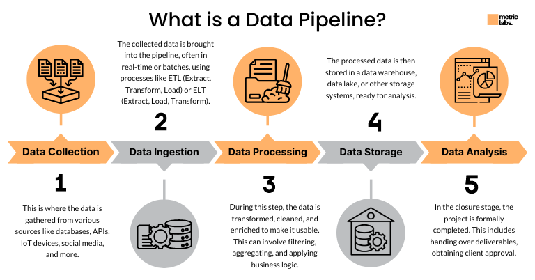
Data Pipeline
A data pipeline is the flow of data from source to target; it is typically automated for efficiency, scalability, and governance (Figure 19.1).
Based on the type of data and the operation of the pipeline we can distinguish
Batch processing pipelines
Stream processing pipelines
ETL (extract-transform-load) pipelines (see Section 19.5)
ELT (extract-load-transform) pipelines (see Section 19.5)
Replication and CDC pipelines
Data Replication
Data replication is the process of creating and maintaining copies of data across multiple locations, systems, or storage devices to ensure availability, improve performance, and provide redundancy. The primary goal is to keep multiple copies of the same data synchronized across different environments.
Replication can be synchronous when changes are written simultaneously to all replicas, or asynchronous when changes are written first to a primary system and later propagated to the replicas.
Change Data Capture (CDC)
Change data capture is a technique for identifying and capturing changes made to data in a database or data source, then delivering those changes to downstream systems; preferably in near real-time. CDC focuses on capturing only the delta (changes) rather than entire data sets. CDC is often the technology that enables efficient data replication. Rather than copying entire databases or tables, CDC identifies the deltas that need to be replicated to keep copies in sync.
Trigger-based CDC uses database triggers to capture changes. It can track very granular changes but requires deep database integration. Many CDC methods are instead log-based, reading the database transaction logs to identify changes in the data. Log-based CDC is non-intrusive, it only requires access to logs, but can reflect only changes that are logged by the database.
Data Lineage
Data lineage refers to tracking the journey of data from origin through transformations. Data lineage is the journey and lifecycle of data as it flows through an organization’s systems, documenting where data originates, how it moves and transforms through various processes, and where it ends up. It provides a comprehensive map of the data path from source to consumption.
Physical lineage tracks the technical movements of data, with a focus on the physical implementation details.
Logical lineage describes what happens to the data from a business perspective, without focus on technical details.
Customer Email Information ↓ [Data Standardization Process] ↓ [Email Validation and Cleansing] ↓ [Customer Master Data Integration]Customer Contact Repository
Metadata
Metadata is often described as “data about the data”. It comes in different flavors.
Technical metadata: describes the structure of the data system such as table names, column names, relationships, file names and sizes, file formats, directory structures, API endpoint definitions, request/response schemas.
Table: customers├── customer_id (INTEGER, PRIMARY KEY, NOT NULL)├── first_name (VARCHAR(50), NOT NULL)├── email (VARCHAR(100), UNIQUE)└── created_date (TIMESTAMP, DEFAULT CURRENT_TIMESTAMP)
Descriptive metadata: provides context that helps discover the data. Examples are column descriptions, data dictionaries, tags and keywords, categories and subject classifications, known quality issues, recommended use cases.
Dataset: sales_transactions├── Description: "Daily sales data from all retail channels"├── Tags: ["sales", "revenue", "daily", "retail"]├── Data Freshness: "Updated nightly at 2 AM EST"├── Known Issues: "Returns data delayed by 24-48 hours"└── Recommended For: "Daily sales reporting, trend analysis"
Business metadata: provides context about what the data means from a business perspective. Examples include non-technical description of data elements, business rules, validation criteria, acceptable ranges, units of measurement, data ownership, data stewards, criticality level.
Field: annual_revenue├── Business Definition: "Total company revenue for the fiscal year"├── Unit: "USD"├── Business Owner: "CFO Office"├── Data Steward: "Financial Planning Team"├── Valid Range: "$0 to $50 billion"└── Update Frequency: "Annually after audit completion"
Operational metadata: tracks how data moves through systems and how it is processed over time. This includes data lineage, source and target systems, transformations and applied business logic, ETL/ELT job execution, processing volumes and performance metrics, data quality scores, etc.
Data Pipeline: customer_daily_load├── Source: CRM_Database.customers├── Last Run: 2024-06-18 02:15:23├── Records Processed: 145,892├── Quality Score: 98.7%├── Processing Time: 12 minutes└── Target: DataWarehouse.dim_customer
Governance metadata: supports data management policies, and compliance with regulatory requirements. Examples are data retention policies, backup and archival rules, user roles, permission matrices, data access policies, version control.
Dataset: customer_personal_data├── Retention Policy: "7 years after last transaction"├── Privacy Classification: "PII - EU residents subject to GDPR"├── Access Level: "Restricted - Marketing team read-only"├── Masking Rule: "Hash email addresses in non-production"└── Compliance: "Annual audit required"
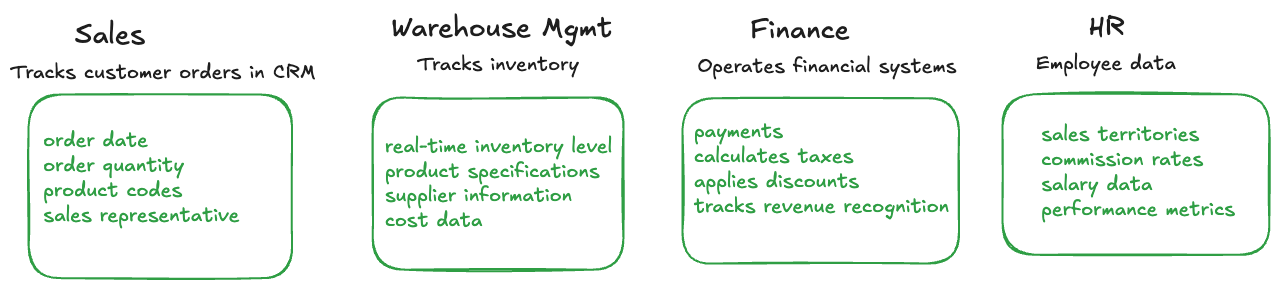
Modern organizations typically run multiple specialized systems that handle different aspects of their business operations. An ERP integration scenario brings together data from these disparate systems to create a unified view of business performance. Consider a mid-sized manufacturing company that uses separate systems for sales management (CRM), inventory control, financial accounting, and human resources.
The sales team uses a CRM system to track customer orders, recording details like order dates, quantities, product codes, and assigned sales representatives. Meanwhile, the warehouse management system maintains real-time inventory levels, product specifications, supplier information, and cost data. The finance department operates a financial system that processes payments, calculates taxes, applies discounts, and tracks revenue recognition. Finally, the HR system stores employee information including sales territories, commission rates, salary data, and performance metrics.
Figure 19.2: ERP integration example
Business Value
Once integrated, these data enable business insights that were not possible with the individual, siloed, systems. Sales managers can see which products are most profitable, not just which generate the most revenue. Territory performance can be measured not just by sales volume but by profitability and customer satisfaction. Financial forecasting becomes more accurate by incorporating sales pipeline data with historical payment patterns.
The integration also supports operational improvements like automatic reorder triggers based on sales velocity, commission calculations that reflect actual profitability rather than just revenue, and customer lifetime value analysis that considers purchase history and payment behavior. Regulatory reporting becomes streamlined when all relevant financial, sales, and employee data can be pulled from a single integrated source.
Challenges
Data Format Inconsistencies
Each system stores dates differently—the CRM might use MM/DD/YYYY format while the financial system uses YYYY-MM-DD. Product identifiers might be stored as “PROD-001” in inventory but “P001” in sales records. Currency fields may have different precision levels across systems.
Timing and Synchronization Issues
Orders are created in the CRM system, but payment processing happens days later in the financial system. Inventory levels update in real-time, but sales reports are generated monthly. This creates challenges in determining accurate profit margins and inventory impacts at any given moment.
Business Logic Complexity
Calculating accurate sales performance requires combining data from all systems. Total order value comes from sales quantities and prices, but profit calculation needs cost data from inventory. Sales representative commissions depend on both sales totals and HR commission rates. Tax calculations vary by customer location and product type.
Data Quality Issues
Sales representatives might enter customer IDs inconsistently, leading to duplicate customer records. Product codes might exist in sales orders but not in the current inventory system due to discontinued items. Employee records might be outdated if someone left the company but still appears in historical sales data.
Referential Integrity Problems
A sales order might reference a customer ID that does not exist in the current customer master data. Financial transactions might link to order numbers that cannot be found in the sales system due to data archiving or system migrations.
Implementation
This scenario typically requires an ETL approach where data is extracted from each source system during off-peak hours, transformed to resolve format inconsistencies and apply business logic, then loaded into a data warehouse optimized for analytical queries. The transformation layer handles currency conversion, date standardization, customer deduplication, and complex calculations like profit margins and commission structures. For more background on ETL versus ELT systems, see Section 19.5 later in this chapter.
19.4 Scenario: Supply Chain Integration
Supply chain integration represents one of the most complex data integration challenges in modern business, involving the seamless connection of data flows across multiple organizations, geographic locations, and disparate technological systems. Consider a global consumer electronics manufacturer that sources components from dozens of suppliers across different countries, operates manufacturing facilities on multiple continents, and distributes products through various retail channels to reach end customers.
The supply chain ecosystem includes primary suppliers who provide critical components like semiconductors and displays, secondary suppliers who manufacture packaging materials and accessories, third-party logistics providers who handle transportation and warehousing, manufacturing facilities with their own production planning systems, quality control laboratories with testing equipment, customs and regulatory systems for international trade, and various retail partners ranging from large big-box stores to small specialty retailers.
Business Value
Successful supply chain integration delivers business value beyond operational efficiency.
Real-time visibility enables just-in-time manufacturing approaches that significantly reduce working capital requirements. Predictive analytics based on integrated supplier data can forecast potential disruptions weeks in advance, allowing proactive mitigation strategies.
Cost optimization becomes possible when procurement teams have integrated views of supplier performance, quality metrics, and total cost of ownership rather than just unit prices.
Sustainability reporting increasingly requires detailed tracking of environmental impacts across the entire supply chain, which is only possible with comprehensive data integration.
Risk management capabilities are dramatically enhanced when the organization can model various disruption scenarios using real supplier data, geographic constraints, and alternative sourcing options. This enables more resilient supply chain design and faster response to unexpected events like natural disasters, political instability, or pandemic-related disruptions.
Data Complexity and Sources
Each participant in this supply chain operates their own systems with unique data formats, update frequencies, and business processes. Suppliers maintain their own inventory management systems, often using different product coding schemes, measurement units, and quality specifications. A semiconductor supplier might track components by wafer lot numbers and electrical specifications, while a packaging supplier focuses on material types, dimensions, and environmental certifications.
Logistics providers generate vast amounts of real-time tracking data including GPS coordinates, temperature readings for sensitive components, customs clearance status, and delivery confirmations. This data comes in various formats—some providers offer modern REST APIs with JSON responses, others still use EDI (Electronic Data Interchange) transactions over legacy networks, and smaller regional carriers might only provide basic email notifications or PDF documents.
Manufacturing facilities produce detailed production data including machine performance metrics, quality test results, yield rates, and material consumption tracking. This operational data is typically stored in Manufacturing Execution Systems (MES) or Enterprise Resource Planning (ERP) systems that may be decades old and use proprietary data formats.
Challenges
External Data Source Management
Unlike internal ERP integration where you control all systems, supply chain integration requires working with external partners who may be unwilling or unable to modify their systems. A key supplier might only provide inventory updates twice daily via CSV files uploaded to an FTP server, while
production needs require real-time visibility. Negotiating data sharing agreements, establishing secure connectivity, and managing different time zones for data updates creates operational complexity.
Data Quality and Reliability Variations Different organizations have varying levels of data maturity and quality controls. A large multinational supplier might provide high-quality, well-structured data with comprehensive metadata, while a smaller regional supplier might send manually-created spreadsheets with inconsistent formatting and frequent errors. The integration system must be robust enough to handle both scenarios while maintaining overall visibility into the supply chain.
Semantic Data Differences
The same concept may be represented differently across organizations. “Lead time” might mean manufacturing time to one supplier, total time including shipping to another, and time from order placement to delivery for a third. Product specifications use different units of measurement, quality standards vary by country, and even basic concepts like “in stock” versus “available to promise” can have different interpretations.
Security and Compliance Complexity
Supply chain data often includes sensitive commercial information like pricing, capacity constraints, and future product roadmaps. Different countries have varying regulations about data residency, encryption requirements, and cross-border data transfers. Integrating this data requires sophisticated security controls, audit trails, and compliance monitoring across multiple jurisdictions.
Dynamic Network Changes
Supply chains constantly evolve as new suppliers are onboarded, existing relationships end, seasonal capacity changes occur, and geopolitical factors impact sourcing decisions. The integration architecture must accommodate these changes without requiring extensive reconfiguration or downtime.
Real-World Operational Scenarios
During normal operations, the integration system continuously monitors supplier inventory levels, production schedules, and shipment status to provide early warning of potential disruptions. When a critical component supplier experiences a production delay, the system must quickly identify alternative suppliers, calculate impact on manufacturing schedules, and automatically trigger rebalancing of orders across the supplier network.
Quality issues create particularly complex integration challenges. When a defective component batch is discovered, the system must trace the affected materials backward through the supply chain to identify the root cause and forward through manufacturing and distribution to determine which finished products might be impacted. This requires maintaining detailed lineage tracking across multiple organizations and systems.
Demand planning scenarios require integrating historical sales data, current inventory positions, supplier capacity constraints, and market forecasts to optimize purchasing decisions. The integration system must handle seasonal patterns, promotional impacts, new product introductions, and economic factors that affect both demand and supply.
Technical Considerations
Supply chain integration typically requires hybrid architectures that combine real-time streaming for critical operational data with batch processing for analytical and planning applications. APIs and messaging systems handle time-sensitive information like shipment tracking and production alerts, while data warehouses store historical information for trend analysis and strategic planning.
The integration platform must support multiple data exchange protocols to accommodate different supplier capabilities, from modern cloud-based APIs to legacy EDI systems. Data transformation capabilities need to handle format conversion, unit standardization, currency conversion, and time zone adjustments across global operations.
Master data management becomes crucial for maintaining consistent product catalogs, supplier information, and location hierarchies across the extended supply chain network. Without proper master data governance, seemingly simple questions like “how much inventory do we have globally for product X” become impossible to answer accurately.
19.5 Enterprise Data Architecture
In larger organizations data are housed in systems with different operational characteristics and various levels of data integration. The key terms you will come across are the data warehouse, the data mart, the data lake, and more recently, the warehouse–lake combination, the lakehouse.
Systems of Record and Operational Systems
These data systems need to be distinguished from systems of records (SoR) and operational systems. A SoR is the authoritative source for a particular piece of data within an organization. It is the designated system where the data are originally created and maintained—it is the single source of truth for the datum. Operational systems support the day-to-day operations of the organizations with functions such as transaction processing, high-frequency updates, ACID compliance.
There is an obvious connection between systems of record and operational systems because SoRs handle live business transactions where the data originates and maintain up-to-date information. Many SoRs are operational systems, but an operational system is not necessarily a system of record. For example, an Oracle database is an operational system, whether it is a system of record depends on the type of data stored in the database. A backup system supports operations but is not the authoritative source of data. A cache system is operational but temporary.
You will also encounter specific system of record–operation system combinations. Salesforce, for example, is a system of record for customer and sales data (CRM, customer relationship management). SAP provides enterprise resource planning (ERP) software that functions as a system of record for financial data and transactions. Workday is a system of record for human resource information.
In summary, the defining characteristic of a system of record is authority and trust. It is the system where data are most accurate and reliable. The defining characteristic of an operational system is its function; how it supports daily business operations. The two concepts overlap significantly but aren’t identical.
Data warehouses and data lakes are generally not systems of records. They contain copies of data that originated in other systems. The focus of the data warehouse is integration of data from multiple sources to support analytics and reporting.
Data warehouses and data lakes represent two distinct philosophies to store data and to make it available in enterprises. Many organizations have both a data warehouse and a data lake, some enterprises have several of each. The data lakehouse is a recent development aimed at combining the pros of warehouses and lakes into a single architecture.
ETL and the Data Warehouse
A data warehouse contains structured data for business intelligence, reporting, and visualization. Data warehouses are updated with data from systems of record and operational source systems such as CRM, ERP, Salesforce on a regular schedule. The main purpose of the data warehouse is querying and analytic processing. It is optimized for query performance, not transformation processing.
The main differences between a data warehouse, also called an enterprise data warehouse (EDW), and a data lake are the level of data curation, the storage technology, and the level of access. The data in data warehouses is highly organized and curated and access to it tends to be more tightly controlled than in a data lake. Data are loaded into a structured data warehouse with predefined schemas (a schema-on-write architecture).
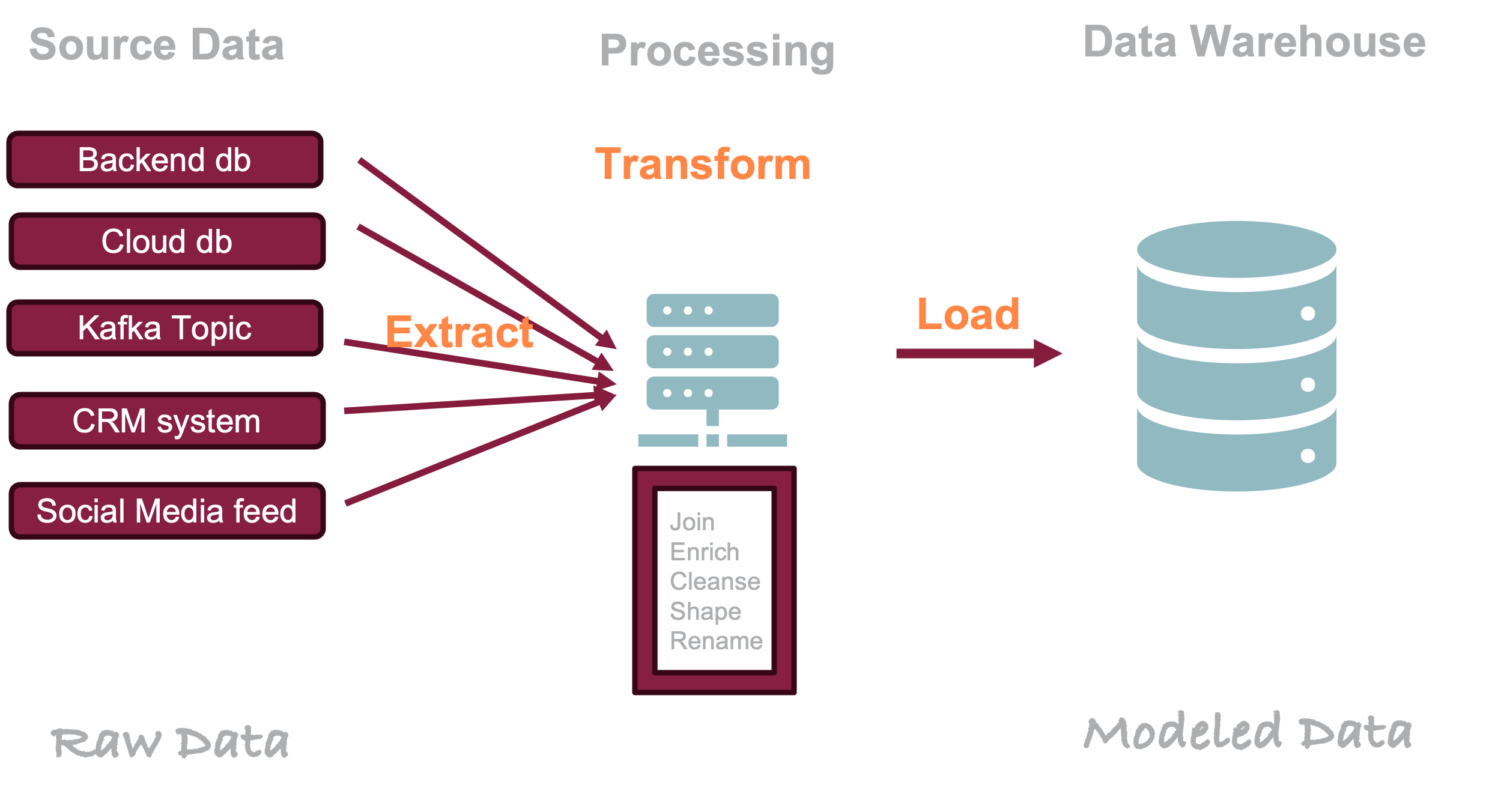
The ETL acronym stands for extract-transform-load, a processing paradigm that describes how the data warehouse is populated. The three phases relate to moving data from a source, performing transformations and integrations and making it available (loading) it in a target system. The stages are
Extract: retrieve data from source systems
Transform: convert data to target format and apply business rules
Load: insert transformed data into target system, here a data warehouse.
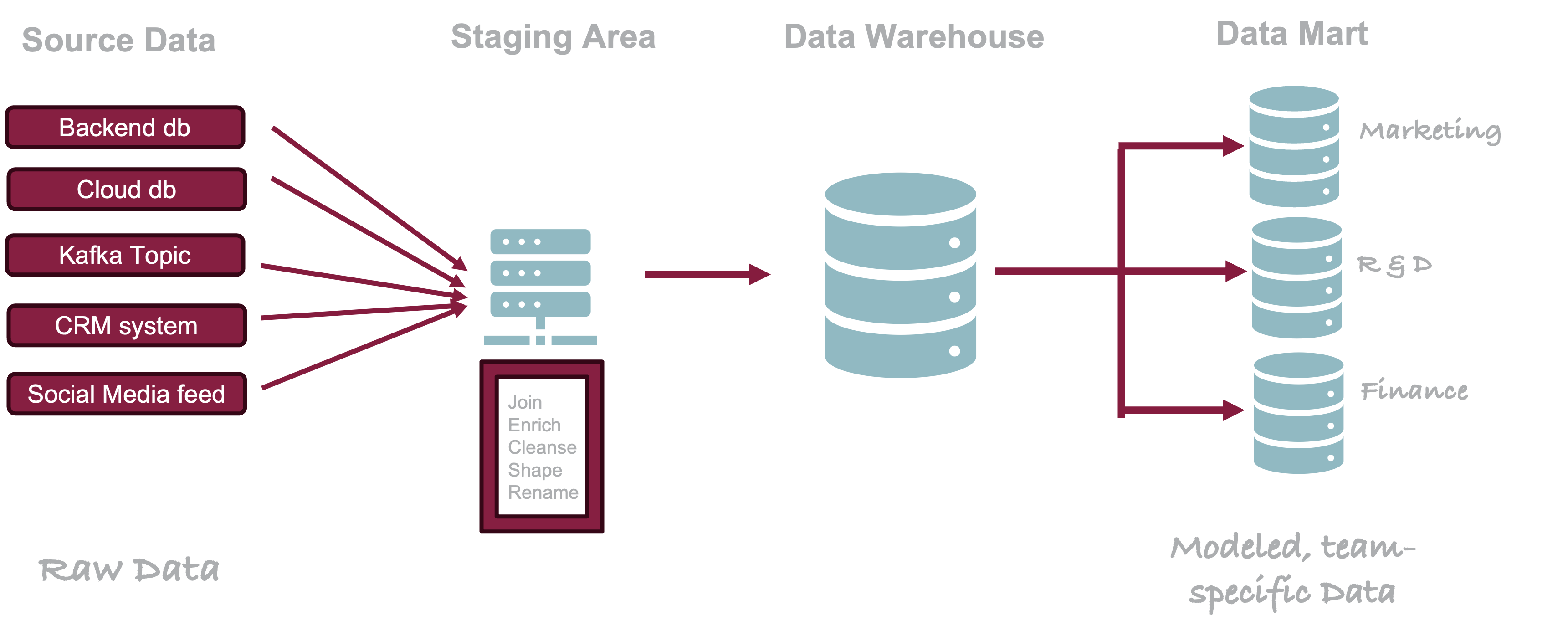
ETL is the traditional paradigm and the target system is a data warehouse (Figure 19.3).
Figure 19.3: Extract-Transform-Load (ELT) paradigm to populate an enterprise data warehouse (EDW).
Extraction of data from a source system can be done by complete copy, incremental change data capture, or real-time streaming. The data lands in a staging server where data are processed (cleansed, validated, converted) and enriched (new columns). Much of data integration happens in the staging area, labeled “Processing” in Figure 19.3. Similar to the extraction phase, the loading of transformed data into the warehouse can be done by copying and replacing entire data sets, incrementally adding only new or updating changed records, or appending records without updating existing ones.
The staging server of the ETL approach presents a bottleneck; its through-put affects the overall performance of the architecture. An alternative to using staging servers is to transform and integrate data in memory during the transfer using beefy large memory machines. The downside of the in-memory approach is limited options for recovery should a machine go down.
Another criticism of the ETL approach is that the data transformation happen prior to loading the EDW. Analysts are limited in what they can do with the data in the warehouse based on what was loaded. If you want to make further transformations or add new features the data needs to be pulled from the EDW or changed in the EDW (frowned upon by the IT department maintaining the EDW).
Schema-on-write
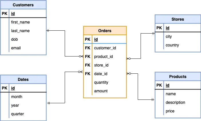
ETL data warehouses consist of schema-on-write tables—dimension and fact tables—and indexes that support consistency (ACID) and are optimized for analytical queries. Fact tables hold numerical data and primary keys; the dimension tables hold the descriptive information for all fields included in a fact table. A typical example is to store orders in a fact table and customers and products information in dimension tables. When relations between the fact and dimension tables are represented by a single join, the arrangement is called a star schema due to the central role of the fact table.
Figure 19.4: One fact table (Orders) and four dimension tables in a star schema. PK denotes primary keys, FK denotes foreign keys. The fact table has foreign keys that support relations with the dimension table. Source.
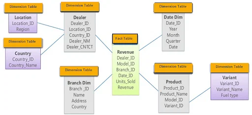
The star schema is one of the simplest ways of organizing data in a data warehouse. The snowflake schema has a more complex structure with normalized dimension tables (without duplicates) and possibly multiple levels of joins.
Figure 19.5: Snowflake schema with up to two levels of relational joins. Source.
The snowflake schema in the preceding figure can require two levels of table joins to query data. For example, to calculate revenue by country requires a join of the fact table with the join of the Dealer and Country tables. In a star schema the location and country information would be incorporated into the Dealer table; that would increase the size of that dimension table due to multiple locations within countries and multiple dealers at locations, but it would simplify the relationship among the tables.
Data warehouses uses SQL as the primary interface, are highly relational, ACID compliant, and schema-dependent—these are attributes of relational database management systems. But you should not equate EDWs with any specific RDBMS. Data warehouses are built on relational database technology but not every RDMBS can serve as a data warehouse. Examples of data warehouses include:
Teradata (on-premises) and Teradata Vantage (cloud-based)
Google BigQuery
Amazon Redshift
Microsoft SQL Server
Oracle Exadata
IBM Db2 and IBM Infosphere
IBM Netezza
SAP/HANA and SAP Datasphere
Snowflake
Yellowbrick
ETL tools and technologies
Traditional ETL Tools
Informatica PowerCenter: Enterprise-grade, visual development
IBM DataStage: High-performance, parallel processing
Microsoft SSIS: Integrated with SQL Server ecosystem
Oracle Data Integrator: Metadata-driven, ELT capabilities
Modern ETL Platforms
Talend: Open-source and commercial versions
Pentaho Data Integration: Java-based, flexible deployment
Apache NiFi: Flow-based, real-time processing
Matillion: Cloud-native, easy-to-use interface
Cloud ETL Services
AWS Glue: Serverless, auto-scaling, managed service
Azure Data Factory: Hybrid integration, visual interface
Google Cloud Dataflow: Stream and batch processing
Snowflake: Built-in transformation capabilities
Data Mart
A data mart is a section of a data warehouse where data is curated for a specific line of business, team, or organizational unit. For example, a data warehouse might contain a data mart for the Marketing organization, a data mart for the R&D organization, and a data mart for the Finance team. These teams have very different needs and different levels of access privileges.
Figure 19.6: A data warehouses supports different data marts. The teams access their data marts rather than the data warehouse directly.
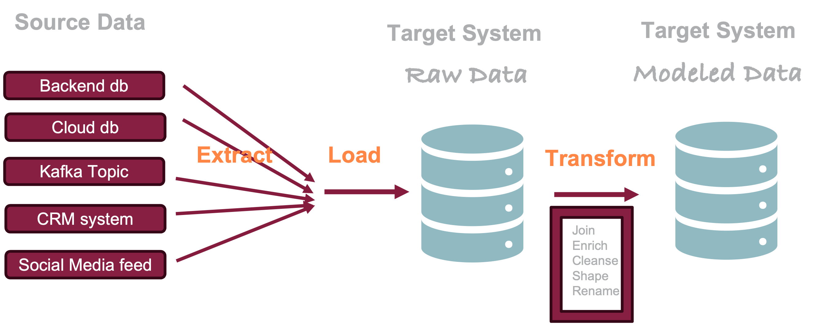
The ELT Approach
The rigid structure of ETL with the data warehouse as the target system does not work well for data scientists building statistical learning models. The approach is more experimental and iterative than standard querying and business reporting—the main purpose of the EDW.
The ELT (extract-load-transform) approach changes the order of the load and transform phases. It does not seem like a big deal, but it has important implications for the work of the data scientist. Figure 19.7 shows an ELT architecture where the data are loaded directly from the source system into a target system. Transformations and integrations are then performed in the target system itself.
Figure 19.7: Extract-Load-Transform (ELT) paradigm to populate a target environment.
The switch from ETL to ELT is not just a change in the processing order. It is enabled by fundamentally different capabilities of the target system. While a data warehouse could function as the target system of an ELT process, it is more likely to be a system with massively parallel processing capabilities, that can handle raw data transformation efficiently, provides separation of compute and storage, uses schema-on-read to apply structure when the data are accessed, and can handle storage and compute efficiently. Examples of such target platforms are Databricks, Google’s BigQuery, Snowflake, and various data lakes.
An advantage of the ELT paradigm is the availability of raw data in the target system. This enables data scientists to create additional transformations, and to process and engineer features. Schema-on-read allows to use the same data in different applications, without forcing it into a rigid structure that is difficult to modify moving forward. It provides flexibility. The modernization of the ETL into the ELT paradigm went hand in hand with the rise of the data lake architecture.
Table 19.1 compares the ELT and ETL approaches with respect to several attributes.
Table 19.1: Comparison of ETL and ELT approaches
Attribute
ETL
ELT
Impact
Processing Location
Dedicated ETL server
Target database/warehouse
ELT leverages target system’s processing power
Data Storage
Processed, cleaned data are stored
Raw data are preserved
ELT provides greater flexibility through reprocessing
Performance
Limited by ETL staging server
Depends on target system’s parallel processing capabilities
ELT often performs better with large data sets
Time to Insight
Available after complete processing
Raw data immediately available, transformed views created as needed
ELT enables faster access to raw data for exploration
Scalability
Scaling up
Scaling out
ELT scaling more cost effective
Data Governance
Cleaner, more controlled data in target
Requires more governance due to access to raw data
raw data needs to be preserved for compliance/analysis
data sources are diverse: handling various formats and structures
Data Lake
Data warehouses have dominated enterprise data storage and analysis for decades. They are not without drawbacks and their disadvantages were amplified during the rise of Big Data with new data types, new workloads, and the need for more flexibility. Data warehouses are often expensive, custom-built appliances that do not scale out easily. They use read-on-write schemas with proprietary storage formats. First Hadoop with the Hadoop Distributed File System (HDFS) and then cloud object storage (Amazon S3, Azure Blob Storage, Google Cloud Storage) presented a much cheaper storage option to reimagine data storage, data curation, and data access. Open-source data formats such as Parquet, ORC, and Avro presented an alternative to storing data in a proprietary format and promised multi-use of the data.
Data lakes were born as centralized repositories where data is stored in raw form. The name suggests that data are like water in a lake, free flowing.
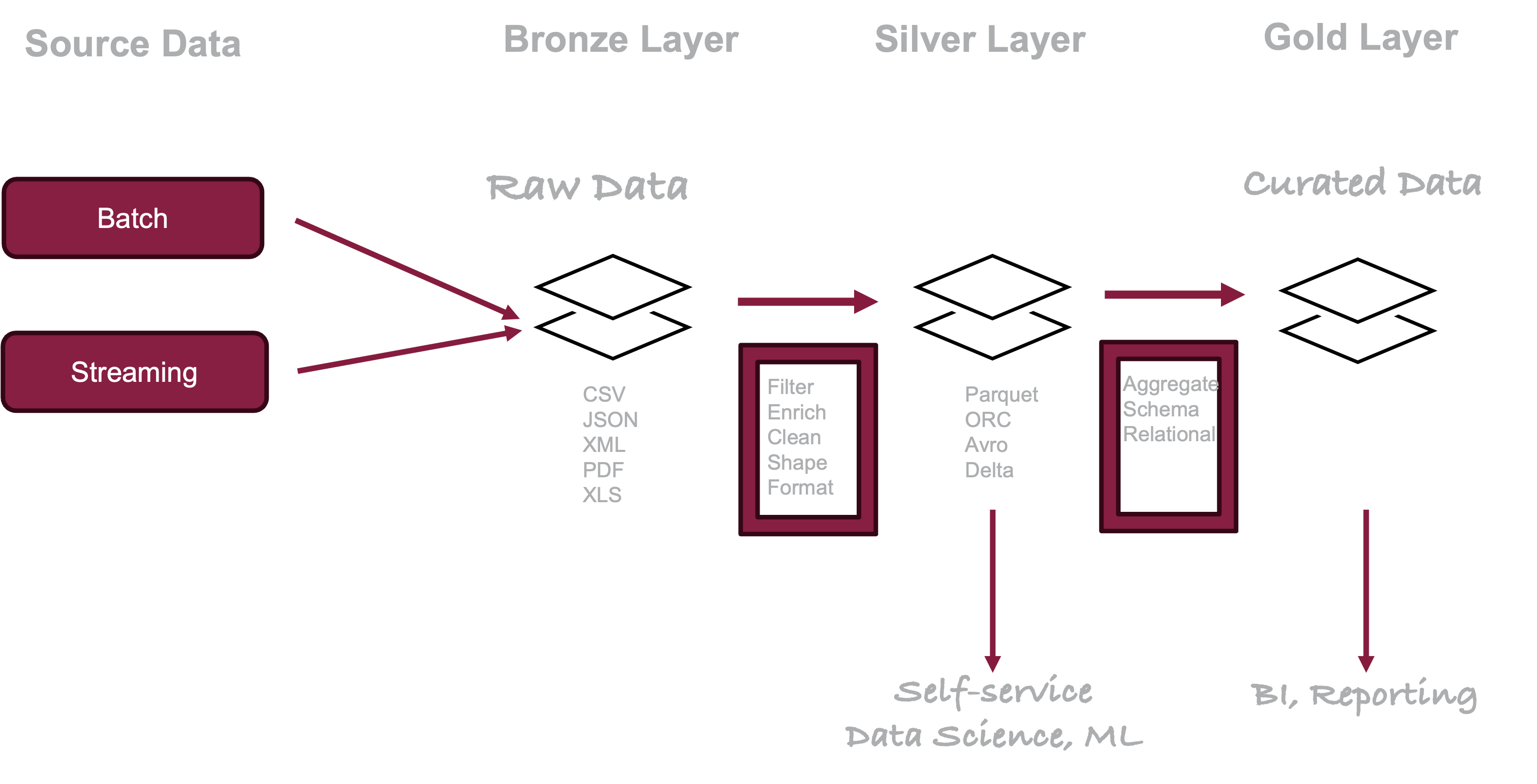
A common data lake architecture is the medallion system named after bronze, silver, and gold medals awarded in competition. The structure and quality improve as one moves from the bronze to the silver to the gold tier. The bronze layer contains the raw data in formats such as CSV, JSON, XML, XLS and is not accessible by the end user. From here the data are cleansed and enriched and formatted into open-source formats such as parquet or Avro. The data in the silver layer is validated and standardized, schemas are defined but can evolve as needed. Users of the silver layer are data scientists and data analysts who perform self-service analysis, data science, and machine learning. Data engineers also use the silver layer to structure and curate data even more for project-specific databases that you find in the gold layer.
Figure 19.8: Medallion data lake design.
The data can be structured, unstructured, or semi-structured. Data lakes support many storage and file formats—CSV, JSON, Parquet, ORC, and Avro are common file formats for data sets. The data is kept in the lake in raw form until it is needed. RDBMS use databases and tables to organize the data. NoSQL databases use document collections and key-value pairs to organize the data. File systems use folders and files to organize files. A data lake uses a flat structure where elements have unique identifiers and are tagged with metadata. Like a NoSQL database, data lakes are schema-on-read systems.
Data lakes are another result of the Big Data era. Increasingly heavy analytical workloads that burned CPU cycles and consumed memory were not welcome in databases and data warehouses that were meant to serve existing business reporting needs. A new data architecture was needed where data scientists and machine learning engineers can go to work, unencumbered by the rigidity of existing data infrastructure and not encumbering the existing data infrastructure with additional number crunching.
The data lake is manifestation of the belief that great insights will (magically) result when you throw together all your data. When data are stored in a data lake without a pre-defined reason and in arbitrary formats, and poorly organized, they can quickly turn into data swamps.
Delta Lake (an open-source metadata layer that sits on top of open file formats like Delta and Parquet)
Data lakes are flexible, scale horizontally (scale-out), and are quite cost effective. They are often built on cheap but scalable object/block/file storage systems that helps reduce costs at the expense of performance. A data warehouse on the other hand is a highly optimized, highly performant system for business intelligence. EDWs often come in the form of packaged appliances (Teradata, Oracle Exadata, IBM Netezza) that makes scaling more difficult. These systems are easier to scale up (adding more memory, more CPUs, etc.) rather than scale horizontally (scale out by adding more machines). EDWs support ACID transactions and allow updates, inserts, and deletes of data. Altering data in a data lake is very difficult, it supports mostly append operations.
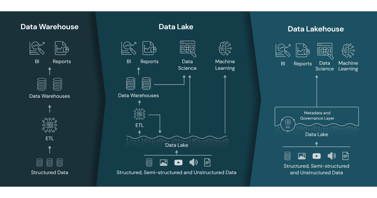
Data science and machine learning is more directed toward the data lake whereas business intelligence is directed at the warehouse. Can the two worlds come together, enabling cost-effective and performant business intelligence and data science on all data in a central place? Maybe. That is the premise and promise of the data lakehouse!
a new, open data management architecture that combines the flexibility, cost-efficiency, and scale of data lakes with the data management and ACID transactions of data warehouses, enabling business intelligence (BI) and machine learning (ML) on all data.
The lakehouse adds a layer on top of the low-cost storage of a data lake that provides data structures and data management akin to a data warehouse.
Figure 19.9: Data warehouse, data lake, and data lakehouse as seen by Databricks. Source.
This is a compelling vision that, if it delivers what it promises, would be a major step into the right direction: to reduce the number of data architectures while enabling more teams to work with data.
It is early days for the data lakehouse but there is considerable momentum. Some vendors are quick to point out that their cloud data warehouses also operate as a lakehouse. Other vendors position SQL query engines on top of S3 object storage as lakehouse solutions. Then there are solutions designed as a data lakehouse, e.g.,
We return to the Enterprise Resource Planning integration example from a previous section and implement the following step in Python:
Working through data integration challenges
Data type inconsistencies
Missing data and referential integrity
data transformation and business logic
data aggregation and summarization
Generating business insights based on the integrated data
Sales by territory
Product performance
Sales rep performance
Commission calculation
Create data quality report
Load the integrated data into a data warehouse
Querying the integrated data in the data warehouse
The sales, warehouse, finance, and HR data would normally come from different data systems. We generate the data on the fly here. As the data warehouse in steps 4. and 5. we choose an in-memory DuckDB database.
print("\n=== DATA INTEGRATION CHALLENGES ===")# Challenge 1: Data Type Inconsistenciesprint("\n1. Data Type Inconsistencies:")print("Sales dates are strings, need conversion to datetime")sales_data['order_date'] = pd.to_datetime(sales_data['order_date'])financial_data['payment_date'] = pd.to_datetime(financial_data['payment_date'])hr_data['hire_date'] = pd.to_datetime(hr_data['hire_date'])print("✓ Date conversions completed")
=== DATA INTEGRATION CHALLENGES ===

1. Data Type Inconsistencies:
Sales dates are strings, need conversion to datetime
✓ Date conversions completed
# Challenge 2: Missing Data and Referential Integrityprint("\n2. Referential Integrity Issues:")print("Checking for orphaned records...")# Check for sales orders without corresponding financial recordsmissing_financial = sales_data[~sales_data['order_id'].isin(financial_data['order_id'])]ifnot missing_financial.empty:print(f"⚠️ Found {len(missing_financial)} sales orders without financial records")else:print("✓ All sales orders have corresponding financial records")# Check for products in sales that don't exist in inventorymissing_products = sales_data[~sales_data['product_id'].isin(inventory_data['product_id'])]ifnot missing_products.empty:print(f"⚠️ Found {len(missing_products)} sales for products not in inventory")else:print("✓ All sold products exist in inventory")
2. Referential Integrity Issues:
Checking for orphaned records...
✓ All sales orders have corresponding financial records
✓ All sold products exist in inventory
# Challenge 3: Data Transformation and Business Logicprint("\n3. Data Transformation and Business Logic:")# Calculate total order valuesales_data['total_order_value'] = sales_data['quantity'] * sales_data['unit_price']print("✓ Calculated total order values")# Calculate profit marginssales_enriched = sales_data.merge(inventory_data[['product_id', 'cost_price']], on='product_id', how='left')sales_enriched['cost_total'] = sales_enriched['quantity'] * sales_enriched['cost_price']sales_enriched['profit'] = sales_enriched['total_order_value'] - sales_enriched['cost_total']sales_enriched['profit_margin'] = (sales_enriched['profit'] / sales_enriched['total_order_value']) *100print("✓ Calculated profit margins")
3. Data Transformation and Business Logic:
✓ Calculated total order values
✓ Calculated profit margins
# Challenge 4: Data Aggregation and Summarizationprint("\n4. Creating Integrated Business Views:")# Create comprehensive sales performance viewintegrated_sales = (sales_enriched .merge(hr_data[['employee_id', 'employee_name', 'territory']], left_on='sales_rep_id', right_on='employee_id', how='left') .merge(financial_data[['order_id', 'payment_status', 'tax_amount', 'discount_amount']], on='order_id', how='left') .merge(inventory_data[['product_id', 'product_name', 'category']], on='product_id', how='left'))print("✓ Created integrated sales performance view")
4. Creating Integrated Business Views:
✓ Created integrated sales performance view
# Generate business insightsprint("\n=== INTEGRATED BUSINESS INSIGHTS ===")# Sales by territoryterritory_sales = integrated_sales.groupby('territory').agg({'total_order_value': 'sum','profit': 'sum','order_id': 'count'}).round(2)territory_sales.columns = ['Total Revenue', 'Total Profit', 'Order Count']print("\n1. Sales Performance by Territory:")print(territory_sales)# Product performanceproduct_performance = integrated_sales.groupby('product_name').agg({'quantity': 'sum','total_order_value': 'sum','profit_margin': 'mean'}).round(2)product_performance.columns = ['Units Sold', 'Revenue', 'Avg Profit Margin %']print("\n2. Product Performance:")print(product_performance)# Sales rep performance with commission calculationrep_performance = integrated_sales.groupby(['sales_rep_id', 'employee_name']).agg({'total_order_value': 'sum','profit': 'sum','order_id': 'count'}).round(2)# Merge with HR data to get commission ratesrep_performance = rep_performance.merge( hr_data[['employee_id', 'commission_rate']], left_index=False, left_on='sales_rep_id', right_on='employee_id', how='left')rep_performance['commission_earned'] = (rep_performance['total_order_value'] * rep_performance['commission_rate']).round(2)print("\n3. Sales Representative Performance:")print(rep_performance[['total_order_value', 'profit', 'order_id', 'commission_earned']])
=== INTEGRATED BUSINESS INSIGHTS ===

1. Sales Performance by Territory:
           Total Revenue  Total Profit  Order Count
territory
East              2400.0         480.0            1
North             3750.0         750.0            2
South             4250.0         850.0            2

2. Product Performance:
                     Units Sold  Revenue  Avg Profit Margin %
product_name
Desktop Workstation          17   4250.0                 20.0
Laptop Pro                   25   3750.0                 20.0
Tablet Ultra                  8   2400.0                 20.0

3. Sales Representative Performance:
   total_order_value  profit  order_id  commission_earned
0             3750.0   750.0         2              187.5
1             4250.0   850.0         2              255.0
2             2400.0   480.0         1               96.0
# Create data quality reportprint("\n=== DATA QUALITY ASSESSMENT ===")def data_quality_report(df, name):"""Generate data quality metrics for a dataset""" total_records =len(df) missing_values = df.isnull().sum().sum() completeness = ((total_records *len(df.columns) - missing_values) / (total_records *len(df.columns)) *100)print(f"\n{name}:")print(f" Total Records: {total_records}")print(f" Missing Values: {missing_values}")print(f" Completeness: {completeness:.1f}%")# Check for duplicates duplicates = df.duplicated().sum()print(f" Duplicate Records: {duplicates}")data_quality_report(sales_data, "Sales Module")data_quality_report(inventory_data, "Inventory Module")data_quality_report(financial_data, "Financial Module")data_quality_report(hr_data, "HR Module")# Demonstrate data lineage trackingprint("\n=== DATA LINEAGE EXAMPLE ===")print("Data transformation pipeline:")print("1. Sales Module → Extract order data")print("2. Inventory Module → Enrich with product details and costs")print("3. Financial Module → Add payment and tax information")print("4. HR Module → Include sales representative details")print("5. Business Logic → Calculate profits, margins, and commissions")print("6. Aggregation → Create territory and product summaries")
=== DATA QUALITY ASSESSMENT ===

Sales Module:
  Total Records: 5
  Missing Values: 0
  Completeness: 100.0%
  Duplicate Records: 0

Inventory Module:
  Total Records: 4
  Missing Values: 0
  Completeness: 100.0%
  Duplicate Records: 0

Financial Module:
  Total Records: 5
  Missing Values: 0
  Completeness: 100.0%
  Duplicate Records: 0

HR Module:
  Total Records: 4
  Missing Values: 0
  Completeness: 100.0%
  Duplicate Records: 0

=== DATA LINEAGE EXAMPLE ===
Data transformation pipeline:
1. Sales Module → Extract order data
2. Inventory Module → Enrich with product details and costs
3. Financial Module → Add payment and tax information
4. HR Module → Include sales representative details
5. Business Logic → Calculate profits, margins, and commissions
6. Aggregation → Create territory and product summaries
import duckdb# create an in-memory databasecon = duckdb.connect(database=':memory:')# Save integrated data (simulating load to data warehouse)print("\n=== SIMULATING DATA WAREHOUSE LOAD ===")# Load data into "data warehouse" tablescon.sql("CREATE OR REPLACE TABLE sales_fact AS SELECT * FROM integrated_sales;")con.sql("CREATE OR REPLACE TABLE territory_summary AS SELECT * FROM territory_sales;")con.sql("CREATE OR REPLACE TABLE product_summary AS SELECT * FROM product_performance;")#integrated_sales.to_sql('sales_fact', engine, if_exists='replace', index=False)#territory_sales.to_sql('territory_summary', engine, if_exists='replace', index=True)#product_performance.to_sql('product_summary', engine, if_exists='replace', index=True)print("✓ Data loaded to data warehouse tables:")print(" - sales_fact (detailed transactions)")print(" - territory_summary (aggregated by territory)")print(" - product_summary (aggregated by product)")
=== SIMULATING DATA WAREHOUSE LOAD ===
✓ Data loaded to data warehouse tables:
  - sales_fact (detailed transactions)
  - territory_summary (aggregated by territory)
  - product_summary (aggregated by product)
# Demonstrate querying the integrated dataprint("\n=== QUERYING INTEGRATED DATA ===")query_string ='''SELECT territory, COUNT(*) as order_count, SUM(total_order_value) as total_revenue, AVG(profit_margin) as avg_margin FROM sales_fact GROUP BY territory ORDER BY total_revenue DESC;'''query_result = con.sql(query_string).df()#query_result = pd.read_sql_query("""# SELECT territory, # COUNT(*) as order_count,# SUM(total_order_value) as total_revenue,# AVG(profit_margin) as avg_margin# FROM sales_fact # GROUP BY territory# ORDER BY total_revenue DESC#""", engine)print("Top performing territories:")print(query_result.round(2))print("\n=== INTEGRATION COMPLETE ===")print("Successfully integrated data from 4 ERP modules:")print("✓ Sales, Inventory, Financial, and HR systems")print("✓ Resolved data quality issues")print("✓ Applied business logic and calculations")print("✓ Created integrated analytical views")print("✓ Loaded to data warehouse for reporting")con.close()
=== QUERYING INTEGRATED DATA ===
Top performing territories:
  territory  order_count  total_revenue  avg_margin
0     South            2         4250.0        20.0
1     North            2         3750.0        20.0
2      East            1         2400.0        20.0

=== INTEGRATION COMPLETE ===
Successfully integrated data from 4 ERP modules:
✓ Sales, Inventory, Financial, and HR systems
✓ Resolved data quality issues
✓ Applied business logic and calculations
✓ Created integrated analytical views
✓ Loaded to data warehouse for reporting