15 SQL Basics
The truth is, most of us learn SQL like we’re learning magic spells.
15.1 Introduction
The question is often asked: “Why should I learn SQL as a data scientist?”. Part of the motivation for the question is that SQL has a reputation as difficult to master, is thought of as dated compared to newer languages like Python, Julia, or Go, and is believed to be the domain of the data base administrator and data engineer.
Figure 15.1 and Figure 15.2 show 2023 results of the annual survey of Master graduates in data science, statistics, and related disciplines, published in the November 2024 issue of Amstat News, the membership magazine of the American Statistical Association.
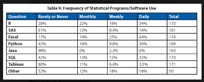
According to Figure 15.1, 44% of the respondents use SQL at least weekly or even daily to perform their work. A third (32%) of the respondents use SQL daily, presumably to interact with data stored in a database. On the flip side, 42% of the respondents sue SQL rarely or never. You either find yourself working for an organization where data scientists encounter no SQL at all or encounter SQL at least once a week.
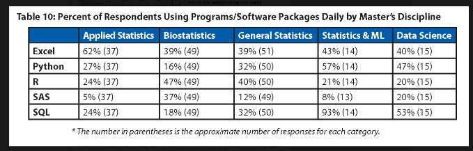
Table 10 of the survey in Figure 15.2 breaks the data down further by disciplines. A stunning 93% of the respondents in Statistics and ML and over 50% of the respondents in the Data Science discipline use SQL every day.
In fact, after the primary programming language (R and Python) and Excel—presumably for receiving data that needs to be processed into a different format—SQL is the most frequently used tool for Master graduates.
This should settle it. Like it or not, SQL is an important tool for (almost) anyone working with data.
SQL is a declarative programming language, you express through programming statements what you want to happen, not how to control the flow of the program. Other examples of declarative languages are CSS, HTML, XML, and Prolog. To support writing scripts, functions, and procedures, database vendors have added flow-control statements (if-then, loops, switches, etc.), but these are extensions of the database and not of the SQL language.
Is it pronounced “S-Q-L” or “sequel”? Both are acceptable but if you want to give a nod to its origin, then you would pronounce it ”sequel” like SEQUEL, the name given to the project by its inventors at IBM in the 1970s. The description as structured query language and the acronym SQL came later.
The concept of a query in SQL is very general: any interaction with a (relational) database. A query in the narrow sense asks questions about the data in the database or retrieves data. Commands that create tables, alter databases, update or delete records, and so on, are also considered queries.
SQL has been standardized and revised since 1986. SQL-92, for example, refers to the revision of the standard in 1992. However, SQL implementations are vendor-specific and do not necessarily comply with any standard. The SQL syntax between databases is similar enough that you can move your SQL code from one dialect to another without too much pain. Moving between databases you will find that the devil is not in the details of the SQL language, but in the details of how NULLs are represented, how date-time values are handled, how indexes work, how data are partitioned, whether foreign keys are supported, and so on. Since we use DuckDB in this chapter, we are following the DuckDB SQL syntax.
SQL has a reputation to be difficult to master. The reputation is not entirely unjustified.
Many programmers are more familiar and comfortable with imperative languages that specify the program flow step by step.
Declarative languages are domain specific, the domain for SQL is the manipulation of data in relational systems. This is associated with a lot of special terminology and domain-specific logic. The data scientist thinks in terms of rows and columns, the database engineer thinks in terms of predicates, projections, clauses, constraints, and relations.
While the number of relevant SQL commands is rather small, SQL queries can become astonishingly complex and unwieldy. A single SQL query that accesses multiple tables with correlated (dependent) subqueries, joins, and common table expressions can be hundreds of lines long. If you are not used to reading SQL, a simple subquery such as this one might give you a headache:
SELECT employee_number, name,
        (SELECT AVG(salary)
           FROM employees
          WHERE department = emp.department) AS department_average
   FROM employees emp
The point of a declarative language is that the programmer specifies the desired result and leaves it to the particular implementation to achieve it. SQL novices often get frustrated because they know exactly what they want but not how to ask for it using SQL syntax.
Debugging SQL code is more difficult than debugging code in an imperative language. Error messages can be cryptic. A query that runs successfully is never wrong from the databases point of view, but it is wrong from the coder’s point of view if it does not produce the desired result. Imagine the surprise if a query runs without error and reports
143,267 records deleted from table foo.- A query that executes quickly for one database can run slowly in another database. Performance depends on database architecture, implementation, optimizations, etc. You must ask for the right\(\texttrademark\) thing in the right\(\texttrademark\) way.
DuckDB CLI
The examples that follow in this section use DuckDB with the ads.ddb database from the command line interface (CLI). The documentation for the CLI is here. You can find installation instructions for the DuckDB clients and your operating system from the installation page.
To invoke DuckDB from the command line with the ads.ddb database use:
> duckdb ads.ddb
D
Three-Valued Logic
An interesting aspect (quirk) of domain-specific logic in SQL is three-valued (ternary) logic. In classical (boolean) logic, there are two logical values, TRUE and FALSE, expressing the relation of a proposition to the truth. In three-valued logic there is a third value, NULL, that expresses some other state. This state can represent not knowable, not yet knowable, irrelevant, uncertain, or undetermined values—it is domain specific. NULL values in databases represent the unknown state of a proposition relative to the truth. This is akin to the concept of a missing value in analytics.
NULL values are not zero or empty values. An empty string (“”) in a text column is a known value, a zero-byte string. A NULL value on the other hand states that a string is absent.
Because NULL is a logical state, SQL defines operations on NULL values. How these operations evaluate is obvious to some and confusing to others. Table 15.1 shows the result of negating a logical value. The “opposite” of NULL is NULL.
| A | NOT A |
|---|---|
| TRUE | FALSE |
| FALSE | TRUE |
| NULL | NULL |
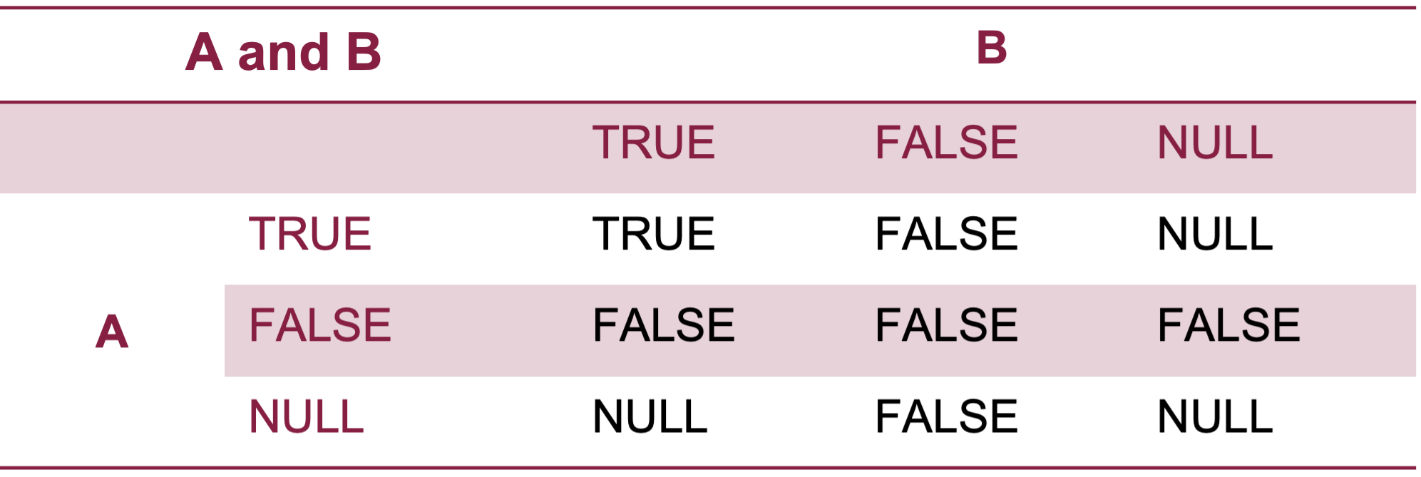
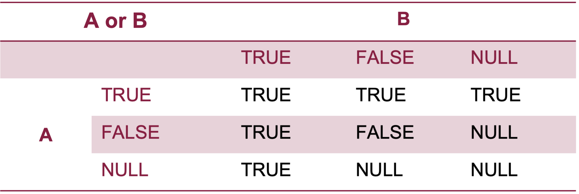
Figure 15.3 and Figure 15.4 display the results of AND and OR operations with logical values. TRUE AND NULL evaluates to NULL, but FALSE AND NULL evaluates to FALSE. TRUE OR NULL evaluates to TRUE, but FALSE OR NULL evaluates to NULL.
To achieve “expected” results when operating on NULL values, special syntax is needed. For example,
SELECT * FROM landsales WHERE improve = NULL;

┌───────┬─────────┬───────┬───────┬───────────┐
│ land  │ improve │ total │ sale  │ appraisal │
│ int64 │  int64  │ int64 │ int64 │  double   │
├─────────────────────────────────────────────┤
│                   0 rows                    │
└─────────────────────────────────────────────┘
returns no rows since the comparison x = NULL is never TRUE, its result is always unknown (NULL). If you use this syntax to check for missing values in your data you will conclude that there are none.
The correct query uses syntax designed to operate with NULL values:
SELECT * FROM landsales WHERE improve IS NULL;
┌───────┬─────────┬───────┬────────┬───────────┐
│ land  │ improve │ total │  sale  │ appraisal │
│ int64 │  int64  │ int64 │ int64  │  double   │
├───────┼─────────┼───────┼────────┼───────────┤
│ 42394 │         │       │ 168000 │           │
│ 93200 │         │       │ 422000 │           │
│ 65376 │         │       │ 286500 │           │
│ 42400 │         │       │        │           │
└───────┴─────────┴───────┴────────┴───────────┘

SELECT count(*) FROM landsales WHERE improve IS NULL;
┌──────────────┐
│ count_star() │
│    int64     │
├──────────────┤
│            4 │
└──────────────┘
15.2 Types of SQL Commands
SQL commands are arranged in logical groups. The most important group for the data scientist is the Data Manipulation Language (DML) group, it consists of statements that change the data stored within a database table and traditionally also includes the most important SQL statement, SELECT. The second most important group of SQL commands is the Data Definition Language (DDL), it provides syntax to create and modify database objects.
Data Definition Language (DDL): syntax to create and modify database objects. The commands are about the objects themselves, not the data they contain. For example, the CREATE TABLE statement defines the schema of a table and creates it, but it does not populate the table with data. Commands in this group include CREATE, DROP, ALTER.
Data Manipulation Language (DML): syntax to query and modify the contents of tables. The most important SQL command in this group is SELECT. Other commands in this group are INSERT, UPDATE, DELETE. The SELECT statement is sometimes pulled into a separate group, the Data Querying Language (DQL). Since it would be the only statement in that group and because SELECT INTO also modifies rows in a table, the SELECT statement is often included as part of the DML.
Data Control Language (DCL): to control access and manage permissions for users of the database. Commands such as GRANT, DENY, and REVOKE are part of the DCL. As a data scientist you are unlikely to work with DCL commands, they are the domain of the database administrator (DBA). However, you might be charged with setting up and maintaining a database and DCL will help you to change what users (or roles) are allowed to do in the database. The following statements allow
user1to run a SELECT statement ontable_foobut disallows updates to the table.
GRANT SELECT ON table_foo TO user1;
DENY UPDATE ON table_foo TO user1;
Not all databases support DCL. SQLite and DuckDB do not because they are embedded databases. They run embedded within the process that launches the database. The process owner has full control over the database, so there is no need to grant, deny, or revoke any access privileges.
15.3 Most Common SQL Commands
The most important SQL commands for a data scientist are the following:
- CREATE TABLE
- ALTER TABLE
- DROP TABLE
- SELECT
- INSERT INTO
- UPDATE
- DELETE FROM
Creating and Modifying a Table
We demonstrate these with a small example using DuckDB. You can find the complete documentation for SQL in DuckDB here. A separate section then dives into the SELECT statement, the workhorse for data analysis in relational DBMS.
First, let’s create a small table with information on some cities around the world.
CREATE TABLE WorldCities (Country VARCHAR, Name VARCHAR, Year INT, Population INT);The table has four columns named Country, Name, Year, and Population, respectively. The first two are of type VARCHAR (allowing character strings of variable length), the last two are of type INT.
If we were to issue the CREATE TABLE statement again, the database would throw an error because the Cities table now exists. To replace an existing table, use CREATE OR REPLACE TABLE:
CREATE OR REPLACE TABLE WorldCities (Country    VARCHAR,
                                     Name       VARCHAR,
                                     Year       INT,
                                     Population INT);
A very useful feature is the addition of check constraints. Suppose you want to make sure that only data after the year 2000 are entered for the Year column. You can add a check constraint like this:
CREATE OR REPLACE TABLE WorldCities (Country    VARCHAR,
                                     Name       VARCHAR,
                                     Year       INT CHECK (Year >= 2000),
                                     Population INT);
Trying to insert a record that fails the check will result in an error:
INSERT INTO WorldCities VALUES ('NL', 'Amsterdam', 1999, 1005);

Error: Constraint Error: CHECK constraint failed: Cities
Once the table exists in the catalog, we can use the ALTER TABLE statement to change its structure, for example, by renaming, adding, or removing columns, changing data types or defaults.
ALTER TABLE WorldCities RENAME Name to CityName;
ALTER TABLE WorldCities ADD Column k INTEGER;
ALTER TABLE WorldCities RENAME to WorldCities;
The first statement renames the Name column to CityName, the second statement adds an integer column named k, and the third statement renames the table.
To populate the table with data, we insert rows. The following statements add one row at a time and then retrieves the entire contents of the table:
INSERT INTO WorldCities VALUES ('NL', 'Amsterdam', 2000, 1005, 1);
INSERT INTO WorldCities VALUES ('NL', 'Amsterdam', 2010, 1065, 3);
INSERT INTO WorldCities VALUES ('NL', 'Amsterdam', 2020, 1158, 4);
INSERT INTO WorldCities VALUES ('US', 'Seattle', 2000, 564, 5432);
INSERT INTO WorldCities VALUES ('US', 'Seattle', 2010, 608, 46);
INSERT INTO WorldCities VALUES ('US', 'Seattle', 2020, 738, 986);
INSERT INTO WorldCities VALUES ('US', 'New York City', 2000, 8015, 0);
INSERT INTO WorldCities VALUES ('US', 'New York City', 2010, 8175, 987);
INSERT INTO WorldCities VALUES ('US', 'New York City', 2020, 8772, 23);

SELECT * FROM WorldCities;
┌─────────┬───────────────┬───────┬────────────┬───────┐
│ Country │ CityName │ Year │ Population │ k │
│ varchar │ varchar │ int32 │ int32 │ int32 │
├─────────┼───────────────┼───────┼────────────┼───────┤
│ NL │ Amsterdam │ 2000 │ 1005 │ 1 │
│ NL │ Amsterdam │ 2010 │ 1065 │ 3 │
│ NL │ Amsterdam │ 2020 │ 1158 │ 4 │
│ US │ Seattle │ 2000 │ 564 │ 5432 │
│ US │ Seattle │ 2010 │ 608 │ 46 │
│ US │ Seattle │ 2020 │ 738 │ 986 │
│ US │ New York City │ 2000 │ 8015 │ 0 │
│ US │ New York City │ 2010 │ 8175 │ 987 │
│ US │ New York City │ 2020 │ 8772 │ 23 │
└─────────┴───────────────┴───────┴────────────┴───────┘ We won’t need the column k anymore, so we can drop it with
ALTER TABLE WorldCities DROP COLUMN k;Pivoting a Table
A pivot table is a summary for data that contains categorical variables. If the aggregation is a simple count, the pivot table is also called a contingency table. These tables are useful to summarize data by categories and to see trends. DuckDB implements the SQL PIVOT statement; the basic syntax is
PIVOT ⟨dataset⟩
  ON ⟨columns⟩
  USING ⟨values⟩
  GROUP BY ⟨rows⟩
  ORDER BY ⟨columns_with_order_directions⟩
  LIMIT ⟨number_of_rows⟩;
The ON clause lists the columns on which to pivot the table. In the WorldCities example we might want to pivot on Year to retrieve the average population for each year:
PIVOT WorldCities on YEAR USING mean(population);┌─────────┬───────────────┬────────┬────────┬────────┐
│ Country │ CityName │ 2000 │ 2010 │ 2020 │
│ varchar │ varchar │ double │ double │ double │
├─────────┼───────────────┼────────┼────────┼────────┤
│ US │ New York City │ 8015.0 │ 8175.0 │ 8772.0 │
│ NL │ Amsterdam │ 1005.0 │ 1065.0 │ 1158.0 │
│ US │ Seattle │ 564.0 │ 608.0 │ 738.0 │
└─────────┴───────────────┴────────┴────────┴────────┘ The USING clause determines how to aggregate the values that are split into columns. If it is not provided, the PIVOT statement defaults to count(*) aggregation.
The GROUP BY clause allows you to further aggregate the results and the ORDER BY statement affects how the output is displayed:
PIVOT WorldCities on YEAR
      USING mean(population)
      GROUP BY Country
      ORDER BY Country DESC;
┌─────────┬────────┬────────┬────────┐
│ Country │ 2000 │ 2010 │ 2020 │
│ varchar │ double │ double │ double │
├─────────┼────────┼────────┼────────┤
│ US │ 4289.5 │ 4391.5 │ 4755.0 │
│ NL │ 1005.0 │ 1065.0 │ 1158.0 │
└─────────┴────────┴────────┴────────┘ To obtain multiple aggregations, provide a list in the USING clause:
PIVOT WorldCities on YEAR
      USING mean(population) as mn,
            max(population) as mx
      GROUP BY Country
      ORDER BY Country DESC;
┌─────────┬─────────┬─────────┬─────────┬─────────┬─────────┬─────────┐
│ Country │ 2000_mn │ 2000_mx │ 2010_mn │ 2010_mx │ 2020_mn │ 2020_mx │
│ varchar │ double │ int32 │ double │ int32 │ double │ int32 │
├─────────┼─────────┼─────────┼─────────┼─────────┼─────────┼─────────┤
│ US │ 4289.5 │ 8015 │ 4391.5 │ 8175 │ 4755.0 │ 8772 │
│ NL │ 1005.0 │ 1005 │ 1065.0 │ 1065 │ 1158.0 │ 1158 │
└─────────┴─────────┴─────────┴─────────┴─────────┴─────────┴─────────┘ You might want to combine creation of a table and populating it with data into a single step. For example, you might want to create a database table from the contents of a CSV file. That is accomplished by adding an AS SELECT clause to the CREATE TABLE statement:
CREATE OR REPLACE TABLE iris AS SELECT * FROM "../datasets/iris.csv”;You can use just FROM as a shorthand for SELECT * FROM:
CREATE OR REPLACE TABLE iris AS FROM "../datasets/iris.csv”;This shorthand works in general in DuckDB:
FROM WorldCities WHERE Country='NL';┌─────────┬───────────┬───────┬────────────┐
│ Country │ CityName │ Year │ Population │
│ varchar │ varchar │ int32 │ int32 │
├─────────┼───────────┼───────┼────────────┤
│ NL │ Amsterdam │ 2000 │ 1005 │
│ NL │ Amsterdam │ 2010 │ 1065 │
│ NL │ Amsterdam │ 2020 │ 1158 │
└─────────┴───────────┴───────┴────────────┘ If you want to create a temporary table that resides in memory and is automatically dropped when the connection to DuckDB is closed, use CREATE TEMP TABLE:
CREATE TEMP TABLE foo AS FROM "../datasets/iris.csv";Dropping a Table
Finally, when the table is no longer needed, we can remove it from the catalog with DROP TABLE:
DROP TABLE WorldCities;15.4 SELECT Statement
The SELECT statement is the workhorse for querying, analyzing, combining, and ordering data in database tables. The more important basic syntax elements of SELECT are
SELECT select_list
   FROM tables
   WHERE condition
   GROUP BY groups
   HAVING group_filter
   ORDER BY order_expr
   LIMIT n;
The logical start of the SELECT query is the FROM clause where you specify the data source for the query. The select_list prior to the FROM clause specifies the columns in the result set of the query. This can be columns from results in the FROM clause, aggregations, and combinations. If you want to specifically name element of the select_list, you can assign an alias with the AS clause, as in this example:
SELECT sepal_length AS SL, sepal_width AS SW from iris LIMIT 5;┌────────┬────────┐
│ SL │ SW │
│ double │ double │
├────────┼────────┤
│ 5.1 │ 3.5 │
│ 4.9 │ 3.0 │
│ 4.7 │ 3.2 │
│ 4.6 │ 3.1 │
│ 5.0 │ 3.6 │
├────────┴────────┤
│ 5 rows │
└─────────────────┘ To include everything in the FROM clause into the select_list, use the asterisk wildcard (star notation):
SELECT * FROM iris LIMIT 4;┌──────────────┬─────────────┬──────────────┬─────────────┬─────────┐
│ sepal_length │ sepal_width │ petal_length │ petal_width │ species │
│ double │ double │ double │ double │ varchar │
├──────────────┼─────────────┼──────────────┼─────────────┼─────────┤
│ 5.1 │ 3.5 │ 1.4 │ 0.2 │ setosa │
│ 4.9 │ 3.0 │ 1.4 │ 0.2 │ setosa │
│ 4.7 │ 3.2 │ 1.3 │ 0.2 │ setosa │
│ 4.6 │ 3.1 │ 1.5 │ 0.2 │ setosa │
└──────────────┴─────────────┴──────────────┴─────────────┴─────────┘ SELECT queries can quickly get complicated because the FROM clause can contain a single table, multiple tables that are joined together, or another SELECT query (this is called a subquery):
SELECT land, improve,
       (SELECT avg(sale) FROM landsales as average)
FROM (SELECT * from landsales where total > 100000);
┌────────┬─────────┬──────────────────────────────────────────────┐
│ land │ improve │ (SELECT avg(sale) FROM landsales AS average) │
│ int64 │ int64 │ double │
├────────┼─────────┼──────────────────────────────────────────────┤
│ 45990 │ 91402 │ 217445.45454545456 │
│ 56658 │ 153806 │ 217445.45454545456 │
│ 51428 │ 72451 │ 217445.45454545456 │
│ 76125 │ 78172 │ 217445.45454545456 │
│ 154360 │ 61934 │ 217445.45454545456 │
│ 40800 │ 92606 │ 217445.45454545456 │
└────────┴─────────┴──────────────────────────────────────────────┘ In the previous SQL code, the select_list contains a SELECT statement that returns the average sale price for all land sales. The FROM clause contains another SELECT statement with a WHERE clause. The result set consists of the land and improvement value for sales where the total value exceeded 100,000 and the average sale for all properties (including the ones with total value below 100,000).
The WHERE clause in the SELECT applies filters to the data. Only rows that match the WHERE clause are processed.
SELECT * FROM iris WHERE species LIKE '%osa' LIMIT 10;┌──────────────┬─────────────┬──────────────┬─────────────┬─────────┐
│ sepal_length │ sepal_width │ petal_length │ petal_width │ species │
│ double │ double │ double │ double │ varchar │
├──────────────┼─────────────┼──────────────┼─────────────┼─────────┤
│ 5.1 │ 3.5 │ 1.4 │ 0.2 │ setosa │
│ 4.9 │ 3.0 │ 1.4 │ 0.2 │ setosa │
│ 4.7 │ 3.2 │ 1.3 │ 0.2 │ setosa │
│ 4.6 │ 3.1 │ 1.5 │ 0.2 │ setosa │
│ 5.0 │ 3.6 │ 1.4 │ 0.2 │ setosa │
│ 5.4 │ 3.9 │ 1.7 │ 0.4 │ setosa │
│ 4.6 │ 3.4 │ 1.4 │ 0.3 │ setosa │
│ 5.0 │ 3.4 │ 1.5 │ 0.2 │ setosa │
│ 4.4 │ 2.9 │ 1.4 │ 0.2 │ setosa │
│ 4.9 │ 3.1 │ 1.5 │ 0.1 │ setosa │
├──────────────┴─────────────┴──────────────┴─────────────┴─────────┤
│ 10 rows 5 columns │
└───────────────────────────────────────────────────────────────────┘ The GROUP BY clause specifies the groupings for aggregations.
SELECT count(*), max(sepal_length) FROM iris GROUP BY species;┌──────────────┬───────────────────┐
│ count_star() │ max(sepal_length) │
│ int64 │ double │
├──────────────┼───────────────────┤
│ 50 │ 7.9 │
│ 50 │ 5.8 │
│ 50 │ 7.0 │
└──────────────┴───────────────────┘ You can specify multiple columns in the grouping or use the GROUP BY ALL shorthand. The following are equivalent:
SELECT League, Division, mean(RBI) FROM Hitters GROUP BY League, Division;
SELECT League, Division, mean(RBI) FROM Hitters GROUP BY ALL;
┌─────────┬──────────┬───────────────────┐
│ League │ Division │ mean(RBI) │
│ varchar │ varchar │ double │
├─────────┼──────────┼───────────────────┤
│ A │ E │ 54.37647058823529 │
│ A │ W │ 48.81111111111111 │
│ N │ E │ 44.94444444444444 │
│ N │ W │ 42.85333333333333 │
└─────────┴──────────┴───────────────────┘The HAVING clause in the SELECT statement causes confusion sometimes, but it is fairly easy to understand as a filter that is applied after the GROUP BY clause. The WHERE clause on the other hand is a filter applied before the GROUP BY clause. In other words, the WHERE clause selects which rows participate in the GROUP BY operation. The HAVING clause determines which results of the GROUP BY operation are filtered.
SELECT League, Division,
       count(*) as count,
       avg(RBI) AS average
FROM Hitters
GROUP BY ALL
HAVING count > 80;

┌─────────┬──────────┬───────┬───────────────────┐
│ League  │ Division │ count │      average      │
│ varchar │ varchar  │ int64 │      double       │
├─────────┼──────────┼───────┼───────────────────┤
│ A       │ E        │    85 │ 54.37647058823529 │
│ A       │ W        │    90 │ 48.81111111111111 │
└─────────┴──────────┴───────┴───────────────────┘
Without the HAVING clause, the SELECT statement would return results on two additional groupings:
SELECT League, Division,
       count(*) as count,
       avg(RBI) AS average
FROM Hitters
GROUP BY ALL;
┌─────────┬──────────┬───────┬───────────────────┐
│ League │ Division │ count │ average │
│ varchar │ varchar │ int64 │ double │
├─────────┼──────────┼───────┼───────────────────┤
│ A │ E │ 85 │ 54.37647058823529 │
│ A │ W │ 90 │ 48.81111111111111 │
│ N │ E │ 72 │ 44.94444444444444 │
│ N │ W │ 75 │ 42.85333333333333 │
└─────────┴──────────┴───────┴───────────────────┘ The ORDER BY and LIMIT clause also operate on the result set of the query. LIMIT is applied at the end of the query and returns only a specified number of rows in the result set. The ORDER BY clause affects how the rows of the result set are arranged. LIMIT without an ORDER BY can be non-deterministic, multiple runs can produce different results depending on the parallel processing of the data. However, combining ORDER BY and LIMIT generates reproducible results and is a common technique to fetch the top or bottom rows. The following SELECT statement retrieves statistics for the baseball players with the five highest RBI values:
SELECT AtBat, Hits, HmRun, Runs, RBI, Walks, Errors
   FROM Hitters ORDER BY RBI DESC LIMIT 5;

┌───────┬───────┬───────┬───────┬───────┬───────┬────────┐
│ AtBat │ Hits  │ HmRun │ Runs  │  RBI  │ Walks │ Errors │
│ int64 │ int64 │ int64 │ int64 │ int64 │ int64 │ int64  │
├───────┼───────┼───────┼───────┼───────┼───────┼────────┤
│   663 │   200 │    29 │   108 │   121 │    32 │      6 │
│   600 │   144 │    33 │    85 │   117 │    65 │     14 │
│   637 │   174 │    31 │    89 │   116 │    56 │      9 │
│   677 │   238 │    31 │   117 │   113 │    53 │      6 │
│   618 │   200 │    20 │    98 │   110 │    62 │      8 │
└───────┴───────┴───────┴───────┴───────┴───────┴────────┘
15.5 Subqueries
A subquery is a query inside another query. The subquery is also called the inner query and the query containing it is referred to as the outer query. Subqueries are said to be uncorrelated if they are self-contained and can be run without the outer query. For example, the following SQL statement contains an uncorrelated subquery, select min(weight) from auto, which you can run as a stand-alone query
SELECT name FROM auto WHERE weight = (SELECT MIN(weight) FROM auto);┌─────────────┐
│ name │
│ varchar │
├─────────────┤
│ datsun 1200 │
└─────────────┘ The outer query in this example is SELECT name FROM auto WHERE weight =.
You can use subqueries together with SELECT EXISTS to test for the existence of rows in the subquery:
SELECT EXISTS(SELECT * FROM auto WHERE horsepower > 300);┌─────────────────────────────────────────────────────┐
│ EXISTS(SELECT * FROM auto WHERE (horsepower > 300)) │
│ boolean │
├─────────────────────────────────────────────────────┤
│ false │
└─────────────────────────────────────────────────────┘A subquery is said to be correlated if the subquery uses values from the outer query. You can think of the subquery as a function that is run for every row in the data. Suppose we want to find the minimum reaction time for each subject in the sleep table. The data represent reaction times for 18 subjects measured on ten days of a sleep deprivation study.
SELECT *
  FROM sleep AS s
  WHERE Reaction =
      (SELECT MIN(Reaction)
       FROM sleep
       WHERE sleep.Subject=s.Subject);
┌──────────┬───────┬─────────┐
│ Reaction │ Days │ Subject │
│ double │ int64 │ int64 │
├──────────┼───────┼─────────┤
│ 249.56 │ 0 │ 308 │
│ 202.9778 │ 2 │ 309 │
│ 194.3322 │ 1 │ 310 │
│ 280.2396 │ 6 │ 330 │
│ 285.0 │ 1 │ 331 │
│ 234.8606 │ 0 │ 332 │
│ 276.7693 │ 2 │ 333 │
│ 243.3647 │ 2 │ 334 │
│ 235.311 │ 7 │ 335 │
│ 291.6112 │ 2 │ 337 │
│ 230.3167 │ 1 │ 349 │
│ 243.4543 │ 1 │ 350 │
│ 250.5265 │ 0 │ 351 │
│ 221.6771 │ 0 │ 352 │
│ 257.2424 │ 2 │ 369 │
│ 225.264 │ 0 │ 370 │
│ 259.2658 │ 6 │ 371 │
│ 269.4117 │ 0 │ 372 │
├──────────┴───────┴─────────┤
│ 18 rows 3 columns │
└────────────────────────────┘ Subject 308 has the smallest reaction time on day 0 of the study, subject 309 has the smallest reaction time at day 2, and so forth. The subquery is correlated, because it uses the column s.Subject from the outer query.
We could have achieved the same aggregation of smallest reaction time by subject with a simple query with GROUP BY clause:
SELECT min(Reaction), Subject FROM sleep GROUP BY subject LIMIT 5;┌───────────────┬─────────┐
│ min(Reaction) │ Subject │
│ double │ int64 │
├───────────────┼─────────┤
│ 249.56 │ 308 │
│ 202.9778 │ 309 │
│ 194.3322 │ 310 │
│ 280.2396 │ 330 │
│ 285.0 │ 331 │
└─────────────────────────┘ The difference is that the correlated subquery returns actual records from the table whereas the SELECT with GROUP BY clause returns the result of aggregation. Put it another way: do you want to see the min reaction time for each subject or do you want to see the records that match the min reaction time for each subject?
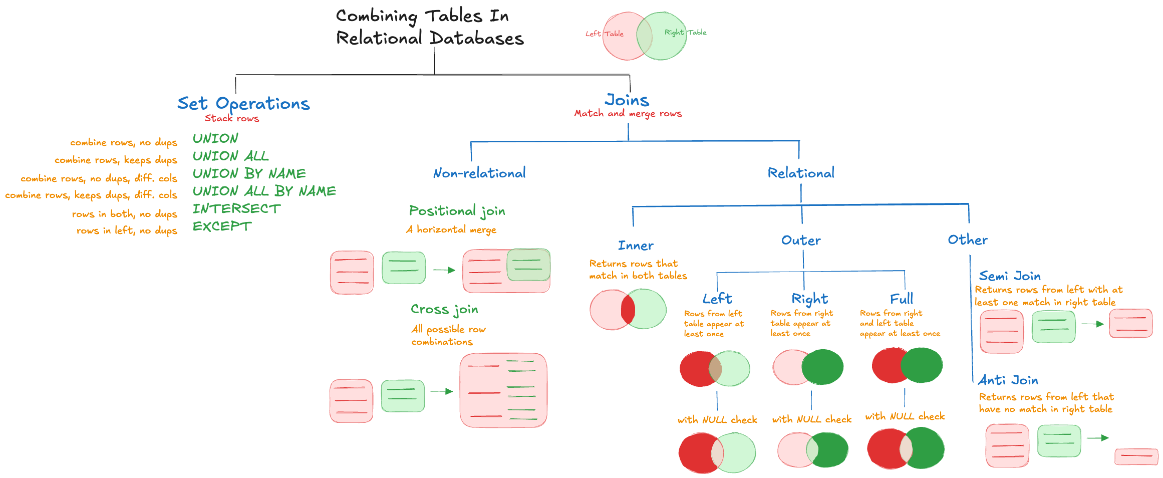
15.6 Combining Tables
The process of combining tables is part of data integration, discussed more fully in Chapter 19. It is based on set operations and joins.
Set operations combine rows of tables without considering the values in the columns. No relationships between the tables are needed, no keys are examined for matches. What happens to columns that exist in one table but not in the other during the append depends on the implementation and the SQL command used. Similarly, what happens to columns that share the same name when tables are merged horizontally depends on the implementation.
A join uses the values in specific columns of the tables to match records.
Figure 15.5 displays the basic (and many) ways two tables can be combined in a relational database system.
Set Operations
We draw on an example in the DuckDB documentation to explain how tables can be merged by rows or columns. First, let’s create two small tables with information on cities:
CREATE TABLE capitals(city VARCHAR, country VARCHAR);
INSERT INTO capitals VALUES ('Amsterdam', 'NL'), ('Berlin', 'Germany');

CREATE TABLE weather(city VARCHAR, degrees INTEGER, date DATE);
INSERT INTO weather VALUES ('Amsterdam', 10, '2022-10-14'),
                           ('Seattle', 8, '2022-10-12');
FROM capitals;
┌───────────┬─────────┐
│ city │ country │
│ varchar │ varchar │
├───────────┼─────────┤
│ Amsterdam │ NL │
│ Berlin │ Germany │
└───────────┴─────────┘FROM weather;
┌───────────┬─────────┬────────────┐
│ city │ degrees │ date │
│ varchar │ int32 │ date │
├───────────┼─────────┼────────────┤
│ Amsterdam │ 10 │ 2022-10-14 │
│ Seattle │ 8 │ 2022-10-12 │
└───────────┴─────────┴────────────┘ Set operations involve two SELECT queries. The queries are connected with clauses that control how the rows are combined:
- UNION: combines rows from queries that have the same columns (number and types) and eliminates duplicates.
- UNION ALL: combines rows from queries that have the same columns (number and types) and preserves duplicates.
- INTERSECT: selects rows that occur in both queries and removes duplicates.
- EXCEPT: selects rows that occur in the left query and removes duplicates.
- UNION BY NAME: works like UNION but does not require the queries to have the same number and types of columns. Eliminates duplicates, like UNION.
- UNION ALL BY NAME: works like UNION BY NAME but does not eliminate duplicate rows.
Here are the result of UNION and UNION ALL clauses:
SELECT city FROM capitals UNION SELECT city FROM weather;

┌───────────┐
│   city    │
│  varchar  │
├───────────┤
│ Amsterdam │
│ Seattle   │
│ Berlin    │
└───────────┘
SELECT city FROM capitals UNION ALL SELECT city FROM weather;
┌───────────┐
│ city │
│ varchar │
├───────────┤
│ Amsterdam │
│ Berlin │
│ Amsterdam │
│ Seattle │
└───────────┘ Here are the results of INTERSECT and EXCEPT clauses:
SELECT city FROM capitals INTERSECT SELECT city FROM weather;

┌───────────┐
│   city    │
│  varchar  │
├───────────┤
│ Amsterdam │
└───────────┘
SELECT city FROM capitals EXCEPT SELECT city FROM weather;
┌─────────┐
│ city │
│ varchar │
├─────────┤
│ Berlin │
└─────────┘ Notice that UNION, UNION ALL, INTERSECT, and EXCEPT require the two queries to return the same columns. The horizontal column matching is done by position. To merge rows across tables with different columns, use UNION (ALL) BY NAME:
SELECT * FROM capitals UNION BY NAME SELECT * FROM weather;

┌───────────┬─────────┬─────────┬────────────┐
│   city    │ country │ degrees │    date    │
│  varchar  │ varchar │  int32  │    date    │
├───────────┼─────────┼─────────┼────────────┤
│ Amsterdam │ NL      │         │            │
│ Seattle   │         │       8 │ 2022-10-12 │
│ Berlin    │ Germany │         │            │
│ Amsterdam │         │      10 │ 2022-10-14 │
└───────────┴─────────┴─────────┴────────────┘
Joins
The previous set operations combine rows of data (vertically). To combine tables horizontally we use join operations. Joins typically are based on the values in columns of the tables to find matches. There are two exceptions, positional and cross joins.
Positional join
For data scientists working with rectangular data frames in which observations have a natural order, merging data horizontally is a standard operation. In relational databases this is a somewhat unnatural operation because relational tables do not work from a natural ordering of the data, they are based on keys and indices. The positional join matches row-by-row such that rows from both tables appear at least once:
select capitals.*, weather.* from capitals positional join weather;

┌───────────┬─────────┬───────────┬─────────┬────────────┐
│   city    │ country │   city    │ degrees │    date    │
│  varchar  │ varchar │  varchar  │  int32  │    date    │
├───────────┼─────────┼───────────┼─────────┼────────────┤
│ Amsterdam │ NL      │ Amsterdam │      10 │ 2022-10-14 │
│ Berlin    │ Germany │ Seattle   │       8 │ 2022-10-12 │
└───────────┴─────────┴───────────┴─────────┴────────────┘
Cross join
The cross join is the simplest join, it returns all possible pairs of rows:
select capitals.*, weather.* from capitals cross join weather;

┌───────────┬─────────┬───────────┬─────────┬────────────┐
│   city    │ country │   city    │ degrees │    date    │
│  varchar  │ varchar │  varchar  │  int32  │    date    │
├───────────┼─────────┼───────────┼─────────┼────────────┤
│ Amsterdam │ NL      │ Amsterdam │      10 │ 2022-10-14 │
│ Amsterdam │ NL      │ Seattle   │       8 │ 2022-10-12 │
│ Berlin    │ Germany │ Amsterdam │      10 │ 2022-10-14 │
│ Berlin    │ Germany │ Seattle   │       8 │ 2022-10-12 │
└───────────┴─────────┴───────────┴─────────┴────────────┘
Inner and outer joins
The two tables in a join are called the left and right sides of the relation. Joins are categorized as outer or inner joins depending on whether rows with matches are returned. An inner join returns only rows that match in the left and right tables of the join. In DuckDB, it is the default join type if you do not qualify the specific join type. Outer joins return rows that do not have any matches; they are further classified as (see Figure 15.5)
- Left outer join: all rows from the left side of the relation appear at least once.
- Right outer join: all rows from the right side of the relation appear at least once.
- Full outer join: all rows from both sides of the relation appear at least once.
To demonstrate the joins in DuckDB, let’s set up some simple tables:
CREATE OR REPLACE TABLE weather (
      city           VARCHAR,
      temp_lo        INTEGER, -- minimum temperature on a day
      temp_hi        INTEGER, -- maximum temperature on a day
      prcp           REAL,
      date           DATE
  );
CREATE OR REPLACE TABLE cities (
      name            VARCHAR,
      lat             DECIMAL,
      lon             DECIMAL
  );
INSERT INTO weather VALUES ('San Francisco', 46, 50, 0.25, '1994-11-27');
INSERT INTO weather (city, temp_lo, temp_hi, prcp, date)
      VALUES ('San Francisco', 43, 57, 0.0, '1994-11-29');
INSERT INTO weather (date, city, temp_hi, temp_lo)
      VALUES ('1994-11-29', 'Hayward', 54, 37);
FROM weather;
┌───────────────┬─────────┬─────────┬───────┬────────────┐
│ city │ temp_lo │ temp_hi │ prcp │ date │
│ varchar │ int32 │ int32 │ float │ date │
├───────────────┼─────────┼─────────┼───────┼────────────┤
│ San Francisco │ 46 │ 50 │ 0.25 │ 1994-11-27 │
│ San Francisco │ 43 │ 57 │ 0.0 │ 1994-11-29 │
│ Hayward │ 37 │ 54 │ │ 1994-11-29 │
└───────────────┴─────────┴─────────┴───────┴────────────┘ INSERT INTO cities VALUES ('San Francisco', -194.0, 53.0);
FROM cities;
┌───────────────┬───────────────┬───────────────┐
│ name │ lat │ lon │
│ varchar │ decimal(18,3) │ decimal(18,3) │
├───────────────┼───────────────┼───────────────┤
│ San Francisco │ -194.000 │ 53.000 │
└───────────────┴───────────────┴───────────────┘ An inner join between the tables on the columns that contain the city names will match the records for San Francisco:
SELECT * FROM weather
         INNER JOIN cities ON (weather.city = cities.name);

┌───────────────┬─────────┬─────────┬───────┬────────────┬───────────────┬───────────────┬───────────────┐
│     city      │ temp_lo │ temp_hi │ prcp  │    date    │     name      │      lat      │      lon      │
│    varchar    │  int32  │  int32  │ float │    date    │    varchar    │ decimal(18,3) │ decimal(18,3) │
├───────────────┼─────────┼─────────┼───────┼────────────┼───────────────┼───────────────┼───────────────┤
│ San Francisco │      46 │      50 │  0.25 │ 1994-11-27 │ San Francisco │      -194.000 │        53.000 │
│ San Francisco │      43 │      57 │   0.0 │ 1994-11-29 │ San Francisco │      -194.000 │        53.000 │
└───────────────┴─────────┴─────────┴───────┴────────────┴───────────────┴───────────────┴───────────────┘
Note that the values for lat and lon are repeated for every row in the weather table that matches the join in the relation. Because this is an inner join (the DuckDB default), and the weather table had no matching row for city Hayward, this city does not appear in the join result. We can change that by modifying the type of join to a left outer join:
SELECT * FROM weather
         LEFT OUTER JOIN cities ON (weather.city = cities.name);

┌───────────────┬─────────┬─────────┬───────┬────────────┬───────────────┬───────────────┬───────────────┐
│     city      │ temp_lo │ temp_hi │ prcp  │    date    │     name      │      lat      │      lon      │
│    varchar    │  int32  │  int32  │ float │    date    │    varchar    │ decimal(18,3) │ decimal(18,3) │
├───────────────┼─────────┼─────────┼───────┼────────────┼───────────────┼───────────────┼───────────────┤
│ San Francisco │      46 │      50 │  0.25 │ 1994-11-27 │ San Francisco │      -194.000 │        53.000 │
│ San Francisco │      43 │      57 │   0.0 │ 1994-11-29 │ San Francisco │      -194.000 │        53.000 │
│ Hayward       │      37 │      54 │       │ 1994-11-29 │               │               │               │
└───────────────┴─────────┴─────────┴───────┴────────────┴───────────────┴───────────────┴───────────────┘
Because the join is an outer join, rows that do not have matches in the relation are returned. Because the outer join is a left join, every row on the left side of the relation is returned (at least once). If you change the left- and right-hand side of the relation you can achieve the same result by using a right outer join:
SELECT * FROM cities
         RIGHT OUTER JOIN weather ON (weather.city = cities.name);

┌───────────────┬───────────────┬───────────────┬───────────────┬─────────┬─────────┬───────┬────────────┐
│     name      │      lat      │      lon      │     city      │ temp_lo │ temp_hi │ prcp  │    date    │
│    varchar    │ decimal(18,3) │ decimal(18,3) │    varchar    │  int32  │  int32  │ float │    date    │
├───────────────┼───────────────┼───────────────┼───────────────┼─────────┼─────────┼───────┼────────────┤
│ San Francisco │      -194.000 │        53.000 │ San Francisco │      46 │      50 │  0.25 │ 1994-11-27 │
│ San Francisco │      -194.000 │        53.000 │ San Francisco │      43 │      57 │   0.0 │ 1994-11-29 │
│               │               │               │ Hayward       │      37 │      54 │       │ 1994-11-29 │
└───────────────┴───────────────┴───────────────┴───────────────┴─────────┴─────────┴───────┴────────────┘
Now let’s add another record to the cities table without a matching record in the weather table:
INSERT INTO cities VALUES ('New York',40.7, -73.9);
FROM cities;

┌───────────────┬───────────────┬───────────────┐
│     name      │      lat      │      lon      │
│    varchar    │ decimal(18,3) │ decimal(18,3) │
├───────────────┼───────────────┼───────────────┤
│ San Francisco │      -194.000 │        53.000 │
│ New York      │        40.700 │       -73.900 │
└───────────────┴───────────────┴───────────────┘
A full outer join between the two tables ensures that rows from both sides of the relation appear at least once:
SELECT * FROM cities
         FULL OUTER JOIN weather ON (weather.city = cities.name);

┌───────────────┬───────────────┬───────────────┬───────────────┬─────────┬─────────┬───────┬────────────┐
│     name      │      lat      │      lon      │     city      │ temp_lo │ temp_hi │ prcp  │    date    │
│    varchar    │ decimal(18,3) │ decimal(18,3) │    varchar    │  int32  │  int32  │ float │    date    │
├───────────────┼───────────────┼───────────────┼───────────────┼─────────┼─────────┼───────┼────────────┤
│ San Francisco │      -194.000 │        53.000 │ San Francisco │      46 │      50 │  0.25 │ 1994-11-27 │
│ San Francisco │      -194.000 │        53.000 │ San Francisco │      43 │      57 │   0.0 │ 1994-11-29 │
│               │               │               │ Hayward       │      37 │      54 │       │ 1994-11-29 │
│ New York      │        40.700 │       -73.900 │               │         │         │       │            │
└───────────────┴───────────────┴───────────────┴───────────────┴─────────┴─────────┴───────┴────────────┘
Semi joins and anti joins
Semi and anti joins are special joins that return rows from only one table in the relation.
A semi join returns rows from the left table that have at least one match in the right table. However, it does not return any rows from the right table.
SELECT * FROM weather
         SEMI JOIN cities ON (weather.city = cities.name);

┌───────────────┬─────────┬─────────┬───────┬────────────┐
│     city      │ temp_lo │ temp_hi │ prcp  │    date    │
│    varchar    │  int32  │  int32  │ float │    date    │
├───────────────┼─────────┼─────────┼───────┼────────────┤
│ San Francisco │      46 │      50 │  0.25 │ 1994-11-27 │
│ San Francisco │      43 │      57 │   0.0 │ 1994-11-29 │
└───────────────┴─────────┴─────────┴───────┴────────────┘
The anti join returns rows from the left table that have no match in the right table:
SELECT * FROM weather
         ANTI JOIN cities ON (weather.city = cities.name);

┌─────────┬─────────┬─────────┬───────┬────────────┐
│  city   │ temp_lo │ temp_hi │ prcp  │    date    │
│ varchar │  int32  │  int32  │ float │    date    │
├─────────┼─────────┼─────────┼───────┼────────────┤
│ Hayward │   37    │   54    │ NULL  │ 1994-11-29 │
└─────────┴─────────┴─────────┴───────┴────────────┘
Joins with NULL checks
The anti join can be used to find records in one table that fail to match records in another table. For example, finding the insurance customers that have never filed a claim—they are absent in the claims table.
Another approach to finding records that do not have a match is to add a NULL check to an outer join. For example, the following statement performs a left outer join and retrieves the records that do not have a match in the right table—as indicated by the WHERE condition cities.name IS NULL.
SELECT * FROM weather
         LEFT OUTER JOIN cities ON (weather.city = cities.name)
         WHERE cities.name IS NULL;

┌─────────┬─────────┬─────────┬───────┬────────────┬─────────┬───────────────┬───────────────┐
│  city   │ temp_lo │ temp_hi │ prcp  │    date    │  name   │      lat      │      lon      │
│ varchar │  int32  │  int32  │ float │    date    │ varchar │ decimal(18,3) │ decimal(18,3) │
├─────────┼─────────┼─────────┼───────┼────────────┼─────────┼───────────────┼───────────────┤
│ Hayward │   37    │   54    │ NULL  │ 1994-11-29 │ NULL    │     NULL      │     NULL      │
└─────────┴─────────┴─────────┴───────┴────────────┴─────────┴───────────────┴───────────────┘
The result is similar to the ANTI JOIN, but the outer join with NULL check returns information from both tables. The anti join only returns information from the left side of the relation.
Similarly, the following query returns the records that have no match in the right side of the relation.
SELECT * FROM cities
       RIGHT OUTER JOIN weather ON (weather.city = cities.name)
       WHERE cities.name IS NULL;

┌─────────┬───────────────┬───────────────┬─────────┬─────────┬─────────┬───────┬────────────┐
│  name   │      lat      │      lon      │  city   │ temp_lo │ temp_hi │ prcp  │    date    │
│ varchar │ decimal(18,3) │ decimal(18,3) │ varchar │  int32  │  int32  │ float │    date    │
├─────────┼───────────────┼───────────────┼─────────┼─────────┼─────────┼───────┼────────────┤
│ NULL    │     NULL      │     NULL      │ Hayward │   37    │   54    │ NULL  │ 1994-11-29 │
└─────────┴───────────────┴───────────────┴─────────┴─────────┴─────────┴───────┴────────────┘
We are done with these two tables, we can drop them from the database.
DROP TABLE cities;
DROP TABLE weather;