38  Data Science Software Engineering

Data science involves statistical programming and writing code. Data scientists are sometimes compared to software engineers and software engineering principles are often applied to data science projects. That is how *agile methodology, continuous integration and deployment, test-driven development, DevOps, and other concepts enter the data science sphere.

But there are substantial difference between data science projects and software engineering projects. Overlooking those differences and forcing standard software engineering workflows onto data science projects contributes to the failure rates in data science.

38.1 Dealing with Uncertainty

The inherent uncertainty and unpredictability of data and the ambiguity of solutions to more open-ended questions are an important difference. Software engineers are comfortable with definite logic, data scientists are comfortable thinking in terms of probabilities.

• Input inherently unpredictable and uncertain. Statistical code is different from non-analytic code in that it is processing an uncertain input. A JSON parser also processes variability, each JSON document is different from the next. Does it not also deal with uncertain input? If the parser is free of bugs, the result of parsing is known with certainty. For example, we are convinced that the sentence “this book is certainly concerned with uncertainty” has been correctly extracted from the JSON file. Assessing the sentiment of the sentence, however, is a data science task: a sentiment model is applied to the text and returns a set of probabilities indicating how likely the model believes the sentiment of the text is negative, neutral, or positive. Subsequent steps taken in the software are based on interpreting what is probable.

• Uncertainty about methods. Whether a software developer uses a quicksort or merge sort algorithm to order an array has impact on the performance of the code but not on the result. Whether you choose a decision tree or a support vector machine to classify the data in the array impacts the performance and the result of the code. A chosen value for a tuning parameter, e.g., the learning rate, can produce stable results with one data set and highly volatile results with another.

• Random elements in code. Further uncertainty is introduced through analytic steps that are themselves random. Splitting data into training and test data sets, creating random folds for cross-validation, drawing bootstrap samples in random forests, random starting values in clustering or neural networks, selecting the predictors in random forests, Monte Carlo estimation, are some examples where data analysis involves drawing random numbers. The statistical programmer needs to ensure that random number sequences that create different numerical results do not affect the quality of the answers. The results are frequently made epeatable by fixing the seed or starting value of the random number generator. While this makes the program flow repeatable, it is yet another quantity that affects the numerical results. It is also a potential source for misuse: “let me see if another seed value produces a smaller prediction error.”

• Data are messy. Data contains missing values and can be full of errors. There is uncertainty about how disparate data sources represent a feature (a customer, a region, a temperature) that affects how you integrate the data sources. These sources of uncertainty can be managed through proper data quality and data integration. As a data scientist you need to be aware and respectful of these issues; they can doom a project if not properly addressed. In an organization without a dedicated data engineering team resolving data quality issues might fall on your shoulders. If you are lucky to work with a data engineering team you still need to be mindful of these challenges and able to confirm that they have been addressed or deal with some of them (missing values).

38.2 Other Differences to Software Engineering

Other differences between data science projects and software engineering projects come to mind.

• Exploration. Data science problems are inherently explorative. Finding insights in data is a discovery operation. While software engineering typically follows defined requirements and specifications, data science projects often start with ambiguous questions that evolve as insights emerge from the data. Software engineering works hard to eliminate ambiguity and uncertainty; data science projects are defined by it.

• Success Criteria. Functionality, performance, reliability, and adherence to requirements are success criteria in traditional software projects. Data science projects add statistical validity, predictive power, and business impact of insights to the list.

• Tooling and Infrastructure. Traditional software development operates with well-established development environments, frameworks, and deployment pipelines. The tooling in data science is more diverse and adds specialized requirements for data management and model deployment.

• Lifecycle. The traditional software development cycle is a more linear progression through development stages. The data science project cycle is highly iterative; earlier stages are revisited frequently as new insights emerge.

• Testing Approach. Traditional software development uses unit tests, integration tests, and functional validation. Testing in data science also includes statistical validation, cross-validation, and prediction-based performance metrics such as precision or recall.

• Programming Languages. Statistical programming uses high-level languages such as R and Python. The software is written at a high level of abstraction, calling into existing packages and libraries. Rather than writing your own implementation of a random forest, you use someone else’s implementation. Instead, your concern shifts to how to use the hyperparameters of the random forest to the greatest effect for the particular data set. You can perform statistical programming in C, C++, or Rust. These system-level languages are best for implementing efficient algorithms, that are then called from a higher-level interface in R or Python.

• Amount of Code. The core modeling functionality of a statistical program is typically short, a few hundred lines long. Include code for data processing, many statistical programs have less than a thousands lines. This is not much compared to the size of large software engineering projects.

• Standalone Programs. A single file or module can contain all the code you need for a statistics project. That is good and bad. Good because it is easy to maintain. Bad because we often skip steps of good software hygiene such as documentation and source control.

---

We discussed in Section 32.1 how MLOps is not just DevOps applied to data science or machine learning. It is its own discipline, based on DevOps, to address the unique challenges of operationalizing machine learning systems at scale. We see from items in the previous list that the same pattern holds for other software engineering concepts: they generally apply but transferal to software using data adds additional challenges.

Another important example is the concept of technical debt.

38.3 Technical Debt

The Concept

The idea of technical debt in software development was introduced by Ward Cunningham, a pioneer in software engineering (Wikis, object-oriented programming, Agile development). He stated at a conference in 1992:

Shipping first-time code is like going into debt. A little debt speeds development so long as it is paid back promptly with refactoring. The danger occurs when the debt is not repaid. Every minute spent on code that is not quite right for the programming task of the moment counts as interest on that debt. Entire engineering organizations can be brought to a stand-still under the debt load of an unfactored implementation, object-oriented or otherwise.

Like borrowing money to invest today with the intent to pay the debt off later, technical debt in software development refers to the design and implementation decisions in favor of expediency in the short term. Like borrowed money that accrues interest until it is repaid, technical debt increases future costs and complexity until the debt is repaid (the technical debt is resolved).

Technical debt is incurred through architecture, structure, duplication, test coverage, code comments and documentation, potential bugs, complexity, or coding practices. Note that not all software issues are technical debt, bugs are quality debt, a delayed feature is feature debt. What all these forms of debt have in common is the accrual of interest, it gets more complicated and expensive to remedy them the longer you wait.

Personal Experience

A typical example of technical debt is choosing an existing technology to build a software solution instead of an emerging technology. Leaning on the current technology is justified because it works, it is well tested, letting others figure out the issues with the new technology, and so on.

Two massive software projects I have worked on created massive technical debt by not incorporating a new technology at the right time.

The first was the emergence of HTML5 at a time when our web applications were redesigned. Arguing that HTML5 was too new and not yet fully proven/vetted/tested, the decision was made to build user interfaces on Adobe Flash/Flex technology instead. Adobe Flash was widely used at the time to create rich web content, Flex (later open-sourced as Apache Flex) was the development framework to build Flash-based applications. HTML5 took off and all major players invested in advancing HTML5. It became the standard for developing web content and eventually Adobe decided to end-of-life the Flash player. This forced us to repay the technical debt before the end-of-life deadline—all web-based user interfaces needed to be reworked to HTML5.

The second example is the use of Python 2 in internal tools. On January 1, 2020, Python 2 was sunset. No further fixes or improvements would be made to the language after that. Python 3 is not backward-compatible with Python 2, there are differences in syntax, exception handling, and so on. We were moving quickly at the time, releasing new software frequently. A rewrite of the internal Python 2 tools would slow that down. Running tools in both Python 2 and Python 3 would also cause additional churn and slowdown. The switch to Python 3 was delayed and every day that passed added more internal code written in Python 2. It is difficult to say in hindsight how invasive (expensive) the move to Python 3 would have been had it been undertaken when Python 3 was first released. When the move finally became absolutely necessary it took about two years to do the switch.

Data Science Solutions

Technical debt is a useful metaphor but its utility is limited by the difficulty to quantify technical debt—unlike financial debt. That a team can move quickly is not evidence of the absence of technical debt. On the contrary, moving quickly might be the reason for increased technical debt.

The concept of technical debt has been applied to fields adjacent to software development, such as information technology (IT). Since data science solutions are software solutions, the concept of technical debt applies to our domain as well. Not treating data science solutions as software engineering projects can be the most expensive technical debt, resulting in solutions that are difficult to maintain and scale over time.

The technical debt in a data science solution might be low if

• It is easy to bring new team member up to speed
• You understand all data dependencies
• You can measure the overall impact to the entire system when changes are made
• You can switch out entire components (such as a model or database) and can estimate the effort to do so
• You can deliver the solution at different scales

As Sculley et al. (2015) argue in their influential paper in the context of machine learning, ML systems (and by extension data science solutions) have a special capacity to incur technical debt. Data science solutions depend on code and have the traditional technical debt issues of software development. In addition, they have data science-specific issues that are difficult to detect and to deal with because these issues exist at the system level rather than the code level. Sculley et al. (2015) organize the system-level interactions in data science (machine learning) systems that contribute to technical debt as follows

1. Erosion of Abstraction Boundaries. The abstraction and encapsulation that makes traditional software robust and invariant does not apply to data-dependent software. It is not invariant to changes in the data.

   • Entanglement. Model inputs are never really independent. Change anything and you change everything (CACE principle). This holds for inputs, optimization settings, hyperparameters, etc.

   • Model Cascades. Training one model based on another model (transfer learning) speeds up training but creates dependencies. Changing the base model in the future is now more difficult, the dependency on the transferred model increases technical debt.

   • Undeclared Consumers. The output of one model is used as input to another system, maybe unbeknownst to the purveyors of the model (a silent consumer). Changing the model reverberates through unexepcted parts of the stack.

2. Data Dependencies. Dependencies in code can be analyzed using static code analysis tools. It is much more difficult to understand how a data science solution depends on data sources.

   • Input data to the model can be unstable and change over time. Even if the data improves, this can negatively affect a deployed model. When the data consumed by the model can be versioned, the data frozen at a particular time point can mitigate the effect of changing inputs.

   • Definition of features can change, for example, when revenue accounting methods change or when a company acquisition introduces a new system for identifying customers, products, regions, etc.

   • The importance of features can erode over time, due to changes in the data and/or because other features have been added to the model.

3. Feedback Loops. Real-time machine learning systems can affect their own behavior if they update over time.

   • Models that impact their future training data can lead to positive (self-fulfilling) or negative (self-defeating) feedback loops. In active learning, for example, you start with a small labeled data set and a large unlabeled data set. A model trained on the labeled data identifies the unlabeled data points where labeling would be most beneficial. Once these are labeled, the training set is increased and the model is retrained. This can lead to selection bias and over-representation of certain data patterns, to reinforcement of existing biases, or models that ignore new patterns in favor of exploiting patterns it handles well.

   • In hidden feedback loops two machine learning systems can influence each other in ways that are difficult to disentangle. Take, for example, two recommendation systems, one (system A) for social media content and one (system B) for news articles. The first recommends based on engagement, the second system based on trendiness. Neither system engages directly with the other. But as system A notices that users engage with certain topics, it recommends more content about these topics. System B notices the topic as trending and promotes related news articles. The two systems operate correctly in isolation, the negative consequences arise when they “work together”; they collaborate inadvertently.

Here are some other examples and sources of technical debt in data science solutions.

• Data Pipelines

  • Brittle ETL processes that break with minor data changes
  • Hard-coded data paths and configurations
  • Missing data validation checks
  • Insufficient error handling for data pipeline failures
  • No monitoring for data drift or quality degradation

• Model Development

  • Undocumented feature engineering decisions
  • Lack of reproducibility in model training
  • Notebook-based development without proper versioning
  • Inconsistent experiment tracking or no experiment management
  • Insufficient test coverage for model performance

• Model Deployment

  • Models deployed without proper CI/CD pipelines
  • Lack of automated retraining procedures
  • Lack of model performance monitoring
  • Poorly documented model dependencies
  • Missing A/B testing infrastructure

• Organizational Factors

  • Siloed knowledge about models or data sources
  • Inconsistent coding standards across data science teams
  • Duplicated efforts due to poor knowledge sharing
  • Inadequate documentation of business requirements and metrics

38.4 Coding Best Practices

Writing code, maintaining code, reviewing code, and fixing code are essential elements of what data professionals do.

Understanding and following best practices is important. 80% of jobs in data science are outside of academic environments. Employers have standard operating procedures (SOPs) for software developers that will apply also to statistical programming and data science projects. For example, many companies use code reviews by fellow developers to evaluate new or modified code before it can be committed to a repository. The feedback from code reviews flows into performance evaluations and has impact on your career. Not following the coding guidelines and best practices of an organization is a great way of shortening tenure. Software projects are collaborative projects and someone else will need to work with your code. How easy is it to understand? Is it well documented? Is it properly structured and modular? How easy is it to debug?

This chapter covers some elementary good coding practices for you to consider.

Software Engineering Principles

Because the result of statistical programming is software, data scientists need to know the principles of good software engineering:

• Modularity: Separate software into components according to functionality and responsibility (functions, modules, public and private interfaces)

• Separation of Concerns: Human beings have a limited capacity to manage contexts. Breaking down a larger task into units and abstractions that you can deal with one at a time is helpful. Interface and implementation are separate concerns. Data quality and data modeling are separate concerns. Not in the sense that they are unrelated, low quality data leads to low quality models—garbage in, garbage out. But in the sense that you can deal with data quality prior to the modeling task. Code efficiency (runtime performance) is sometimes listed as an example for separating concerns: write the code first to meet criteria such as correctness and robustness, then optimize the code for efficiency, focusing on the parts of the code the run spends most time in.

• Abstraction: Separate the behavior of software components from their implementation. Look at each component from two points of views: what it does and how it does it. A client-facing API (Application Programming Interface) specifies what a module does. It does not convey the implementation details. By looking at the function interface of prcomp and princomp in R, you cannot tell that one function is based on singular-value decomposition and the other is based on eigenvalue decomposition.

• Generality: Software should be free from restrictions that limit its use as an automated solution for the problem at hand. Limiting supported data types to doubles and fixed-size strings is convenient, but not sufficiently general to deal with today’s varied data formats (unstructured text, audio, video, etc.). The “Year 2000” issue is a good example of lack of generality that threatened the digital economy: to save memory, years were represented in software products as two-digit numbers, causing havoc when 1999 (“99”) rolled over to “00” on January 1, 2000.

• Anticipation of Change: Software is an automated solution. It is rarely finished on the first go-around; the process is iterative. Starting from client requirements the product evolves in a back and forth between client and developer, each side refining their understanding of the process and the product at each step. Writing software that can easily change is important and often difficult. When software components are tightly coupled and depend on each other, it is unlikely that you can swap out for another without affecting both.

• Consistency: It is easier to do things within a familiar context. Consistent layout of code and user interfaces helps the programmer as well as the user as well as the next programmer. Consistency in code formatting, comments, naming conventions, variable assignments, etc. makes it easier to read and modify code and helps to prevent errors. When you are consistent in initializing all local variables in C functions, you will never have uninitialized variable bugs.

Version Control

Version control refers to the management and tracking of changes in digital content; mostly files and mostly code. Any digital asset can be placed under version control. Even if you are working (mostly) by yourself, using a version control system is important. Employers consider it a non-negotiable skill and you do not want to stand out as the applicant who does not know how to use Git. The benefits of version control systems are many, even the solo programmer would be remiss not to use it.

What does a version control system like Git do for you:

• It keeps track of files and their changes over time.

• It saves changes to files without duplicating the contents, saving space in the process.

• It groups content in logical units (branches) that are managed together. For example, all files associated with a particular build of a software release are kept in a branch.

• It is a time machine, allowing you to reconstruct a previous state of the project and to see the complete history of the files.

• It is a backup machine, making sure you have access to older versions of files and that changes do not get lost.

• It allows you to perform comparisons between versions of files and to reconcile their differences.

• It allows you to safely experiment with code without affecting code others depend on.

• It allows you to see which parts of a project are worked on most/least frequently.

• It is a collaborative tool, that reconciles changes to files made by multiple developers. Version control systems allow you to submit changes to someone else’s code.

• By supporting modern continuous integration/continuous deployment (CI/CD) principles, a version control system can automate the process of testing and deploying software.

The list goes on and on. The main point is that these capabilities and benefits are for everyone, whether you work on a project alone or as a team member.

Tip

Oh how I wish there were easily accessible version control systems when I did my Ph.D. work. It involved a lot of programming algorithms and the analysis of real data sets. Developing the code took months to years and went through many iterations. I made frequent backups of the relevant files using really cool storage technology using special 1GB-size cartridges and a special reader. There were disks labeled “January 1993”, “March 1993”, “December 1993”, “Final”, “Final-V2”, and so forth. The storage technology was discontinued by the manufacturer and the cartridges are useless today. I am not able to access the contents even if the bits have not rotted on the media by now.

To study how the algorithm I needed to write for the dissertation evolved over time, I would have to go through all the backups and compare files one by one. A version control system will show me the entire history of changes in one fell swoop.

Using a cloud-based version control system would have avoided that headache. Alas, that did not exist back then.

There are many version control systems, Git, Perforce, Beanstalk, Mercurial, Bitbucket, Apache Subversion, AWS CodeCommit, CVS (Concurrent Versions System, not the drugstore chain), and others.

The most important system today is Git. GitHub and GitLab are built on top of Git. What is the relationship? Git is a local version control system, it runs entirely on the machine where it is installed and manages file changes there. GitHub and GitLab are cloud-based systems that allow you to work with remote repositories. In addition to supporting Git remotely, GitHub adds many cool features to increase developer productivity. The files for the pages you are reading are managed with Git and stored in a remote repository on GitHub (the URL is https://github.com/oschabenberger/oschabenberger-github.io-bn). GitHub also hosts the web site for the text through GitHub Pages. GitHub Actions can be set up so that the web site (the book) automatically rebuilds if any source files changes. And all of that comes with the free capabilities of GitHub.

A Crash Course in Git

Git is installed on your machine, it is a local tool for versioning files. You can perform all major Git operations (clone, init, add, mv, restore, rm, diff, grep, log, branch, commit merge, rebase, etc.) without an internet connection. The collaborative aspect of version control comes into play when you use a Git service provider such as GitHub or GitLab. Besides making Git a tool for multi-user applications, using GitHub or GitLab also gives you the ability to work with remote repositories; you can push your local changes to a server in the cloud, making it accessible to others and making it independent of the local workstation. Just because you push a repository to GitHub does not necessarily give everyone on the internet access to it—you manage whether a repository is private or public.

Installing Git

There are several ways to get Git on your machine, see here. On MacOS, installing the XCode Command Line tools will drop git on the machine. To see if you already have Git, open a terminal and check:

➜ which git
/usr/bin/git

The executable is installed in /usr/bin/git on my MacBook.

Basic configuration

There are a million of configuration options for Git and its commands. You can see the configuration with

➜ git config --list

To connect to GitHub later, add your username and email address to the configuration:

➜ git config --global user.name "First Last"
➜ git config --global user.email "first.last@example.com"

You can have project-specific configurations, simply remove the --global option and issue the git config command from the project (repository) directory.

Repositories

A repository is a collection of folders and files. Repositories are either cloned from an existing repository or initialized from scratch. To initialize a repository, change into the root directory of the project and issue the git init command:

➜ cd "STAT 5014"
➜ STAT 5014 pwd
/Users/olivers/Documents/Teaching/Data Science/STAT 5014
➜ STAT 5014 git init
Initialized empty Git repository in /Users/olivers/Documents/Teaching/Data Science/STAT 5014/.git/
➜ STAT 5014 git:(main)

To get help on git or any of the git commands, simply add --help:

➜ git --help
➜ git status --help
➜ git add --help

Stages of a file

A file in a Git repository goes through multiple stages (Figure 38.1). At first, the file is unmodified and untracked. A file that was changed in any way is in a modified state. That does not automatically update the repository. In order to commit the change, the file first needs to be staged with the git add command.

When you issue a git add on a new file or directory, it is being tracked. When you clone a repository, all files in your working directory will be tracked and unmodified.

Figure 38.1: The lifecycle of a file in Git. Source

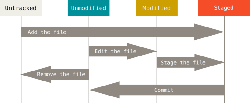
A file that is staged will appear under the “Changes to be committed” heading in the git status output.

Once you commit the file it goes back into an unmodified and tracked state.

Tracking files

To track files in a repository, you need to explicitly add them to the file tree with git add. This does not commit the file or push the file into a branch or a remote repository, it simply informs Git which files you care about.

➜ git add LeastSquares.R
➜ git add *.Rmd
➜ git add docs/

The previous commands added LeastSquares.R, all .Rmd files in the current directory, and all files in the docs subfolder to the Git tree. You can see the state of this tree any time with

➜ git status

git status shows you all files that have changed as well as files that are not tracked by Git and are not ignored. For example, after making some changes to the quarto.yml and to reproducibility.qmd files since the last commit, the status of the repository for this material looks as follows:

➜  StatProgramming git:(main) ✗ git status
On branch main
Your branch is up to date with 'origin/main'.

Changes not staged for commit:
  (use "git add <file>..." to update what will be committed)
  (use "git restore <file>..." to discard changes in working directory)
    modified:   _quarto.yml
    modified:   docs/reproducibility.html
    modified:   docs/search.json
    modified:   reproducibility.qmd

Untracked files:
  (use "git add <file>..." to include in what will be committed)
    .DS_Store
    .gitignore
    .nojekyll
    .python-version
    StatProgramming.Rproj
    _book/
    ads.ddb
    customstyle.scss
    data/
    debug_ada.R
    debug_ada.Rmd
    images/
    latexmacros.tex
    sp_references.bib

no changes added to commit (use "git add" and/or "git commit -a")

Two more files have been noted by Git as modified, docs/reproducibility.html and docs/search.json. These files are generated by Quarto when the content of the modified files is being rendered. They will be added to the next commit to make sure the website is up to date and not just the source (.qmd) files.

git add can be a bit confusing because it appears to perform multiple functions: to track a new file and to stage a file for commit. If you think of git add as adding precisely the content to the next commit, then the multiple functions roll into a single one.

---

An ignored file is one for which you explicitly tell Git not to worry about. You list those files in a .gitignore file. (You can have multiple .gitignore files in the directory hierarchy, refer to the Git documentation on how they interact. The typical scenario is a .gitignore file in the root of the repository.)

The contents of the following .gitignore file state that all .html files should be ignored, except for foo.html. Also, StatLearning.Rproj will be ignored.

➜ cat .gitignore
*.html
!foo.html
StatLearning.Rproj

Files that are listed in .gitignore are not added to the repository and persist when a repository is cloned. However, if a file is already being tracked, then adding it to .gitignore does not untrack the file. To stop tracking a file that is currently tracked, use

git rm --cached filename 

to remove the file from the tree. The file name can then be added to the .gitignore file to stop the file from being reintroduced in later commits.

Files that you want to exclude from tracking are often binary files that are the result of a build or compile, and large files. Also, if you are pushing to a public remote repository, make sure that no files containing sensitive information are added.

Committing changes

Once you track a file, Git keeps track of the changes to the file. Those changes are not reflected in the repository until you commit them with the commit command. A file change will not be committed to the repository unless it has been staged. git add will do that for you.

It is a good practice to add a descriptive message to the commit command that explains what changes are committed to the repository:

➜ git commit -m "Early stopping criterion for GLMM algorithm"

If you do not specify a commit message, Git will open an editor in which you must enter a message.

Tip

If Git opens an editor for you and this is the first time you find yourself in vi or vim, you might struggle with those editors. To set a different default editor on MacOS or Linux, set the EDITOR environment variable.

➜ echo $EDITOR

tells you whether a default text editor has been set.

Since only files that have been added with git add are committed, you can ask Git to notice the changes to the files whose contents are tracked in your working tree and do corresponding git adds for you by adding the -a option to the commit:

➜ git commit -a -m "Early stopping criterion for GLMM algorithm"

What happens when you modify a file after you ran git add but before the net commit? The file will appear in git status as both staged and ready to be committed and as unstaged. The reason is because Git is tracking two versions o f the file now: the state it was in when you first ran git add and the state it is in now, which includes the modifications since the last git add. In order to stage the most recent changes to the file, simply run git add on the file again.

Remote repositories

The full power of Git comes to light when you combine the local work in Git repositories with a cloud-based version control service such as GitHub or GitLab. To use remote repositories with Git, first set up an account, say with GitHub.

The Git commands to interact with a remote repository are

• git pull: Incorporates changes from a remote repository into the current branch. If the current branch is behind the remote, then by default it will fast-forward the current branch to match the remote. The result is a copy of changes into your working directory.

• git fetch: Copies changes from a remote repository into the local Git repository. The difference between fetch and pull is that the latter also copies the changes into your working directory, not just into the local repo.

• git push: Updates remote references using local references, while sending necessary objects.

• git remote: Manage the set of remote repositories whose branches you track.

Note

If you have used other version control systems, you might have come across the terms pushing and pulling files. In CVS, for example, to pull a file means adding it to your local checkout of a branch, to push a file means adding it back to the central repository.

With Git, push and pull command only come into play when you work with remote repositories. As long as everything remains on your machine, you do not need those commands. However, most repositories these days are remote, so the initial interaction with a repository is often a clone, pull, or fetch.

Start by creating a new repository on GitHub by clicking on the New button. You have to decide on a name for the repository and whether it is public or private. Once you created a remote repository, GitHub gives you alternative ways of addressing it, using https, ssh, etc.

Tip

Depending on which type of reference you use on the command line, you also need different ways of authenticating the transaction. GitHub removed passwords as an authentication method for command-line operations some time ago. If you use SSH-style references you authenticate using the passphrase of an SSH key registered with GitHub. If you use https-style references you authenticate with an access token you set up in GitHub.

Back on your local machine you manage the association between the local repository and the remote repository with the git remote commands. For example,

➜ git remote add origin git@github.com:oschabenberger/oschabenberger-github.io-bn.git

associates the remote repository described by the ssh syntax git@github.com:oschabenberger/oschabenberger-github.io-bn.git with the local repository. Using html syntax, the same command looks like this:

➜ git remote add origin https://github.com/oschabenberger/oschabenberger-github.io-bn

GitHub provides these strings to you when you create a repository.

To update the remote repository with the contents of the local repository, issue the git push command:

➜ git push

Structure and Organization

Naming

• Choose names for variables and functions that are easy to understand. Variable and function names should be self explanatory. Most modern programming languages and tools no longer limit the length of function or variable names, there is no excuse for using a1, a2, b3 as variable names. Use nouns for names of variables and objects that describe what the item holds; for example, originalData and randomForestResult instead of d and out.

• Stick with a naming convention such as snake_case, PascalCase, or camelCase. In snake_case, spaces between words are replaced with an underscore. In camelCase, words are concatenated and the first letter of the word is capitalized. PascalCase is a special case where the first letter of the entire name is also capitalized; camelCase is ambivalent about capitalizing the first letter of the name. The following are examples of names in camelCase.

accountBalance
thisVariableIsWrittenInCamelCase
itemNumber
socialSN
MasterCard

An issue with camelCase is that it is not entirely clear how to write names in that style that contain other names or abbreviations, for example, is it NASAAdminFiles or NasaAdminFiles? I am not sure it really matters.

snake_case is popular because it separates words with underscores—mimicking white space—while producing valid names for computer processing. The following are examples of names in snake_case:

account_balance
ACCOUNT_BALANCE
home_page
item_Number

Using upper-case letters in snake_case is called “screaming snake case”, situations where I have seen it used are the definition of global constants or macro names in C. kebab case is similar to snake case but uses a hyphen instead of an underscore. Here are examples of names in kebab case:

account-balance
home-page
item-Number

Although it might look nice, it is a good idea to avoid kebab case in programs. Imagine the mess that ensues if the hyphen were to be interpreted as a minus sign! While the compiler might read the hyphen correctly, the code reviewer in the cubicle down the hall might think it is a minus sign.

Do not assign objects to existing names, unless you really want to override them. This goes in particular for internal symbols and built-in functions. Unfortunately, R does not blink and allows you to do things like this:

T <- runif(20)
C <- summary(lm(y ~ x))

These assignments override the global variable whose value is set to TRUE for logical comparison and the function C() that defines contrasts for factors. If in doubt whether it is safe to assign to a name, check in the console whether the name exists or request help for it

?T
?C()

Comments

Unless you write a literal program use comments throughout to clarify why code is written a certain way and what the code is supposed to accomplish. Even with literal programs, comments associated with code are a good practice because the code-portion of the literal program can get separated from the text material at some later point.

Comments frequently are intended by programmers to leave themselves some notes, for example, about functions yet to be written or to be refactored later. Make it clear with a “TODO” at the beginning of the comment where those sections of the program are and make the TODO comment stand out visually from other comments.

It is a good practice to have a standardized form for writing comments. For example, you can have a standard comment block at the beginning of functions. Some organizations will require you to write very detailed comment blocks that explain all inputs and outputs down to length of vectors and data types.

# -------------------------------------------------------------------
# TODO: Add check whether it is safe to perform the division before
#       returning from the function. Variances can be zero or near zero.
# -------------------------------------------------------------------

# ###################################################################
# Function: getIRLSWeights
# Purpose: retrieve the vector of weights for iteratively 
#          reweighted least squares
# Arguments:
#       eta: numeric vector of linear predictors
#       link: character string describing the link function
#       dist: character string describing the distribution of the response 
#
# Returns: the vector of weights, same length as the eta vector (input)
#
# Notes: 
#   For efficiency, eta is not checked for NULL or missing values. 
#   These checks are in the deta_dmu() and get_var() functions.
# ###################################################################

getIRLSWeights <- function(eta, link="log", dist="poisson") {
    var_z <- deta_dmu(eta,link)^2 * get_var(get_mu(eta,link),dist)
    return (1/var_z)    
}

If you program in Python, you would add docstrings to the function. This also serves as the help information for the user.

Whitespace

Judicious use of whitespace makes code more readable. It helps to differentiate visually and to see patterns. Examples are indentation (use spaces, not tabs), alignment within code blocks, placement of parentheses, and so forth.

Which of the following two functions is easier to read? It does not matter for the R interpreter but it matters for the programmer.

get_z <- function(y, eta, link) {
if (is.null(y) || is.null(eta)) {
stop("null values not allowed") }
if (anyNA(y) || anyNA(eta)) {
stop("cannot handle missing values") }
z <- eta + (y - get_mu(eta,link)) * deta_dmu(eta,link)
return(z)
}

get_z <- function(y, eta, link) {
    if (is.null(y) || is.null(eta)) {
        stop("null values not allowed")
    }
    if (anyNA(y) || anyNA(eta)) {
        stop("cannot handle missing values")
    }
    z <- eta + (y - get_mu(eta,link)) * deta_dmu(eta,link)
    return(z)
}

The following code uses indentation to separate options from values and to isolate the function definition for handling the reference strip. The closing parenthesis is separated with whitespace to visually align with the opening parenthesis of xyplot.

xyplot(diameter ~ measurement | Tree, 
       data    = apples,
       strip   = function(...) {
           # alter the text in the reference strip   
           strip.default(..., 
                         strip.names  = c(T,T), 
                         strip.levels = c(T,T),
                         sep          = " ")
       },
       xlab    = "Measurement index",
       ylab    = "Diameter (inches)",
       type    = c("p"),
       as.table= TRUE,
       layout  = c(4,3,1)
      )

With languages such as Python, where whitespace is functionally relevant, you have to use spacing within the limits of what the language allows.

Functions

R

In R almost everything is a function. When should you write functions instead of one-off lines of code? As always, it depends; a partial answer hides in the question. When you do something only once, then writing a bunch of lines of code instead of packaging the code in a function makes sense. When you write a function you have to think about function arguments (is the string being passed a single string or a vector?), default values, return values, and so on.

However, many programming tasks are not one-offs. Check your own code, you probably write the same two or three “one-off” lines of code over and over again. If you do it more than once, consider writing a function for it. If you do a substantial task over and over, consider writing a package.

Note

If you are interested in writing an R package, check out this chapter in the book by Peng, Kross, and Anderson (2020).

Function names should be verbs associated with the function purpose, e.g., joinTables(), updateWeights(). For functions that retrieve or set values, using get and set is common: getWeights(), setOptimizationInput().

The comment block for function should document the function purpose, required arguments, and returns.

Some argue that it is good coding practice to have default values on function arguments. For example,

addNumbers <- function(a=1, b=2) {return(a+b)}

instead of

addNumbers <- function(a, b) {return(a+b)}

Adding defaults ensures that all variables are initialized with valid values and simplifies calling the function. On the other hand, it can mask important ways to control the behavior of the function. Users will call a function as they see it being used by others and not necessarily look at the function signature. Take the duckload() function:

duckload <- function(tableName, whereClause=NULL, dbName="ads.ddb") {
    if (!is.null(tableName)) {
        if (!("duckdb" %in% (.packages()))) {
            suppressWarnings(library("duckdb"))
            message("duckdb library was loaded to execute duckload().")
        }
        con <- dbConnect(duckdb(), dbdir=dbName, read_only=TRUE)
        query_string <- paste("SELECT * from ", tableName)
        if (!is.null(whereClause)) {
            query_string <- paste(query_string, " WHERE ", whereClause)
        }
        df_ <- dbGetQuery(con, query_string)
        dbDisconnect(con)
        return (df_)
    } else {
        return (NULL)
    }
}

Would you know from the following usage pattern that you can pass a WHERE clause to the SQL string?

duckload("apples")

If the function arguments had no defaults, the function call would reveal its capabilities:

duckload("apples", whereClause=NULL, dbName="ads.ddb")
# or
duckload("apples",NULL,"ads.ddb")

Other good practices to observe when writing functions:

• Always have an explicit return argument. It makes it much easier to figure out where you return from the function and what exactly is being returned.

• Check for NULL inputs

• Check for missing values unless your code can handle them.

• Handle errors (see below)

• Pass through variable arguments (...)

• If you return multiple values, organize them in a list or a data frame. Lists are convenient to collect objects that are of different types and sizes into a single object. The following function returns a list with three elements,

iterationWeight <- function(Gm,wts,method="tree") {
    pclass <- predict(Gm,type="vector")
    misclass <- pclass != Gm$y
    Em <- sum(wts*misclass)/sum(wts)
    alpha_m <- log((1-Em)/Em)
    return (list("misclass"=misclass,"Em"=Em,"alpha_m"=alpha_m))
}

Error Handling

Think of a function as a contract between you and the user. If the user provides specified arguments, the function produces predictable results. What should happen when the user specifies invalid arguments or when the function encounters situations that would create unpredictable results or situations that keep it from continuing?

Your opportunities to handle these situations include issue warning messages with warning(), informational messages with message(), stopping the execution with stop() and stopifnot() and try-catch-finally execution blocks. In general, stopping the execution of a function with stop or stopifnot is a last resort if the function cannot possibly continue. If the data passed are of the wrong type and cannot be coerced into the correct data type, or if coercion would result in something nonsensical, then stop.

In the event that inputs are invalid and you cannot perform the required calculations, could you still return NULL as a result? If so, do not stop the execution of the function. You can issue a warning message and then return NULL. Warning messages are also appropriate when the function behavior is changing in an unexpected way. For example, the input data contains missing values (NAs) and your algorithm cannot handle them. If you process the data after omitting missing values, then issue a warning message if that affects the dimensions of the returned objects.

Keep in mind that R is used in scripts and as an interactive language. Messages from your code are intended for human consumption so they should be explicit and easy to understand. But avoid making your code too chatty.

To check whether input values have the expected types you can use functions such as

is.numeric()
is.character()
is.factor()
is.ordered()
is.vector()
is.matrix()

and to coerce between data types you can use the as. versions

as.numeric()
as.character()
as.factor()
as.ordered()
as.vector()
as.matrix()

tryCatch() is the R implementation of the try-catch-finally logic you might have seen in other languages. It is part of the condition system that provides a mechanism for signaling and handling unusual conditions in programs. tryCatch attempts to evaluate expression expr, and if it succeeds, executes the code in the finally block. You can add erorr and warning handlers with the error= and warning= options.

tryCatch(expr,
         error = function(e){
           message("An error occurred:\n", e)
         },
         warning = function(w){
           message("A warning occured:\n", w)
         },
         finally = {
           message("Finally done!")
         }
        )

tryCatch is an elegant way to handle conditions, but you should not overdo it. It can be a drag on performance. For example, if you require input to be of numeric type, then it is easier and faster to check with is.numeric than to wrap the execution in tryCatch.

Dependencies

It is a good idea to check dependencies in functions. Are the required packages loaded? It is kind of you to load required packages on behave of the caller rather than stopping execution. If you do, issue a message to that effect. See duckload() above for an example.

Installing packages on behalf of the caller is a step too far in my opinion, since you are now changing the R environment. You can check whether a package is installed with require. The following code stops executing if the dplyr package is not installed.

check_pkg_deps <- function() {
    if (!require(dplyr))
        stop("the 'dplyr' package needs to be installed first")
}

require() is similar to library(), but while the latter fails with an error if the package cannot be loaded, require returns TRUE or FALSE depending on whether the library was loaded and does not throw an error if the package cannot be found. Think of require as the version of library you should use inside of functions.

Documentation

Comments in code are not documentation. Documentation is a detailed explanation of the purpose of the code, how it works, how its functions work, their arguments, etc. It also includes all information someone would want to need to take over the project. In literal programs you have the opportunity to write code and documentation at the same time. Many software authoring frameworks include steps in programming that generate the documentation. For example, to add documentation to an R package, you need to create a “man” subdirectory that contains one file per function in the special R Documentation format (.Rd). You can see what the files look like by browsing R packages on GitHub. For example, here is the repository for the ada package.

At a minimum a README file in Markdown should accompany the program. The file has setup instructions and use instructions someone would have to follow to execute the code. It identifies author, version, major revision history, and details on the functions in the public API—those functions called by the user of the program.

There are great automated documentation systems such as doxygen which annotate the source code in such a way that documentation can be extracted automatically. An R package for generating inline documentation that was inspired by doxygen is roxygen2.

Python

Peng, Roger D., Sean Kross, and Brooke Anderson. 2020. Mastering Software Development in r. https://bookdown.org/rdpeng/RProgDA/.

Sculley, D., Gary Holt, Daniel Golovin, Eugene Davydov, Todd Phillips, Dietmar Ebner, Vinay Chaudhary, Michael Young, Jean-Francois Crespo, and Dan Dennison. 2015. “Hidden Technical Debt in Machine Learning Systems.” In Proceedings of the 29th International Conference on Neural Information Processing Systems - Volume 2, 2503–11. NIPS’15. Cambridge, MA, USA: MIT Press.