13 Data Sources and File Formats
13.1 File Formats
If you are working with proprietary data analytics tools such as SAS, SPSS, Stata, or JMP, you probably do not worry much about the ways in which data are stored, read, and written by the software, except that you want the tool to support import to and export from your favorite non-proprietary format.
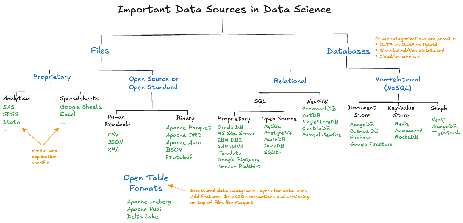
Most data science today is performed on open-source or open standard file formats (Figure 13.1). Proprietary formats are not easily exchanged between tools and applications. Data science spans many technologies and storing data in a form accessible by only a subset of the tools is counterproductive. You end up reformatting the data into an exchangeable format at some point anyway.
The most important file formats in data science are CSV, JSON, Parquet, ORC, and Avro. CSV and JSON are text-based, human-readable formats, whereas Parquet, ORC, and Avro are binary formats. The last three were designed specifically to handle Big Data use cases, Parquet and ORC in particular are associated with the Hadoop ecosystem. Parquet, ORC, and Avro are Apache open-source projects.
Although CSV and JSON are ubiquitous, they were never meant for large data volumes.
You will encounter many other data formats in data science work, but these five file formats cover a lot of ground, you should have a basic understanding of their advantages and disadvantages.
Spreadsheet programs such as Microsoft Office Excel, Google Sheets, Apple Numbers, are everywhere. Excel is one of the most frequently encountered format to communicate data in the corporate world. Unfortunately so.
We discuss below why spreadsheets are not suitable for data science. Many analytic data sets ready for modeling started out as spreadsheets but data science rarely uses the format to store processed data that is ready for modeling. Maybe the best advice we can give about data in spreadsheets is that when you receive data in that format, make the files immutable (read-only) and convert the content as soon as possible into a format suitable for storing analytic data.
CSV
In data science projects you will invariably work with comma-separated values (CSV) files. Not because that is a great file format, but because CSV files are ubiquitous for rectangular data sets made up of rows and columns. Each line of the file stores one record with values in plain text separated by commas.
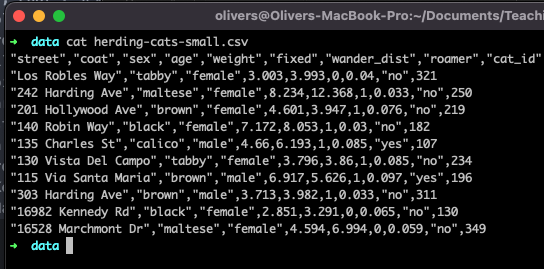
Figure 13.2 shows the contents of a CSV file with ten observations. The first line lists the column names. Strings are enclosed in quotes and values are separated by commas.
Among the advantages of CSV files are
- Ubiquitous: every data tool can read and write CSV files. It is thus a common format to exchange (export/import) data between tools and applications.
- Human readable: since the column names and values are stored in plain text, it is easy to look at the contents of a CSV file. When data are stored in binary form, you need to know exactly how the data are laid out in the file to access it.
- Compression: since the data are stored in plain text it is easy to compress CSV files.
- Excel: CSV files are easily exported from and imported to Microsoft Excel.
- Simple: the structure of the files is straightforward to understand and can represent tabular data well if the data types can be converted to text characters.
There are some considerable disadvantages of CSV files, however:
- Human readable: To prevent exposing the contents of the file you need to use access controls and/or encryption. It is not a recommended file format for sensitive data.
- Simple structure: Complex data types such as documents with multiple fields and sub-fields cannot be stored in CSV files.
- Plain text: Some data types cannot be represented as plain text, for example, images, audio, and video. If you kluge binary data into a text representation the systems writing and reading the data need to know how to kluge and un-kluge the information—it is not a recommended practice.
- Efficiency: much more efficient formats for storing data exist, especially large data sets.
- Broken: CSV files can be easily broken by applications. Examples include inserting line breaks, limiting line width, not handling embedded quotes correctly, blank lines.
- Missing values (NaNs): The writer and reader of CSV files need to agree how to represent missing values and values representing not-a-number. Inconsistency between writing and reading these values can have disastrous results. For example, it is a bad but common practice to code missing values with special numbers such as 99999; how does the application reading the file know this is the code for a missing value?
- Encodings: When CSV files contain more than plain ASCII text, for example, emojis or Unicode characters, the file cannot be read without knowing the correct encoding (UTF-8, UTF-16, EBCDIC, US-ASCII, etc.). Storing encoding information in the header section of the CSV file throws off CSV reader software that does not anticipate the extra information.
- Metadata: The only metadata supported by the CSV format are the column names in the first row of the file. This information is optional and you will find CSV files without column names. Additional metadata common about columns in a table such as data types, format masks, number-to-string maps, cannot be stored in a CSV file.
- Data Types: Data types need to be inferred by the CSV reader software when scanning the file. There is no metadata in the CSV header to identify data types, only column names.
- Loss of Precision: Floating point numbers are usually stored in CSV files with fewer decimal places than their internal representation in the computer. A double-precision floating point number occupies 64-bits (8 bytes) and has 15 digits of precision. Although it is not necessary, floating-point numbers are often rounded or truncated when they are converted to plain text.
Despite these drawbacks, CSV is one of the most common file formats. It is the lowest common denominator format to exchange data between disparate systems.
JSON
JSON stands for JavaScript Object Notation, and although it was borne out of interoperability concerns for JavaScript applications and is based on a JavaScript standard, it is a language-agnostic data format. Initially used to pass information in human readable form between applications over APIs (Application Programmer Interfaces), JSON has grown into a general-purpose format for text-based, structured information. It is the standard for communicating on the web. The correct pronunciation of JSON is apparently akin to the name “Jason”, but “JAY-sawn” has become common.
A binary, non-human readable form of JSON was created at MongoDB and is called BSON (binary JSON).
In contrast to CSV, JSON is not based on rows of data but three basic data elements:
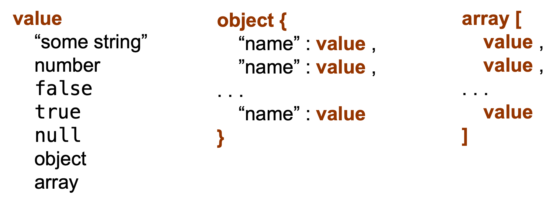
- Value: a string, number, reserved word, or one of the following:
- Object: a collection of name—value pairs similar to a key-value store.
- Array: An ordered list of values
All modern programming languages support key—values and arrays, they might be calling it by different names (object, record, dictionary, struct, list, sequence, map, hash table, …). This makes JSON documents highly interchangeable between programming languages—JSON documents are easy to parse (read) and write by computers. Any modern data processing system can read and write JSON data, making it a frequent choice to share data between systems and applications.
A value in JSON can be a string in double quotes, a number, true, false, or null, an object or an array. Objects are unordered collection of name—value pairs. An array is an ordered collection of values. Since values can contain objects and arrays, JSON allows highly nested data structures that do not fit the row structure of CSV files.
JSON documents are self-describing, the schema to make the data intelligible is built into the structures. It is also a highly flexible format that does not impose any structure on the data, except that it must comply with the JSON rules and data types—JSON is schema-free.

Many databases support JSON as a data type, allowing you to store hierarchical information in a cell of a row-column layout, limited only by the maximum size of a text data type in the database. Non-relational document databases often use JSON as the format for their documents.
Since so much data is stored in JSON format, you need to get familiar and comfortable with working with JSON files. Data science projects are more likely consumers of JSON files rather than producer of files.
Apache Parquet
The Apache Parquet open-source file format is a binary format—data are not stored in plain text but in binary form. Originally conceived as a column-based file format in the Hadoop ecosystem, it has become popular as a general file format for analytical data inside and outside of Hadoop and its file system HDFS: for example, as an efficient analytic file format for data exported to data lakes or in data processing with Spark.
Working with Parquet files for large data is an order of magnitude faster than working with CSV files. The drawbacks of CSV files discussed previously melt away with Parquet files.
Parquet was designed from the ground up with complex data structures and read-heavy analytics in mind. It uses principally columnar storage but does it cleverly by storing chunks of columns in row groups rather than entire columns Figure 13.5).
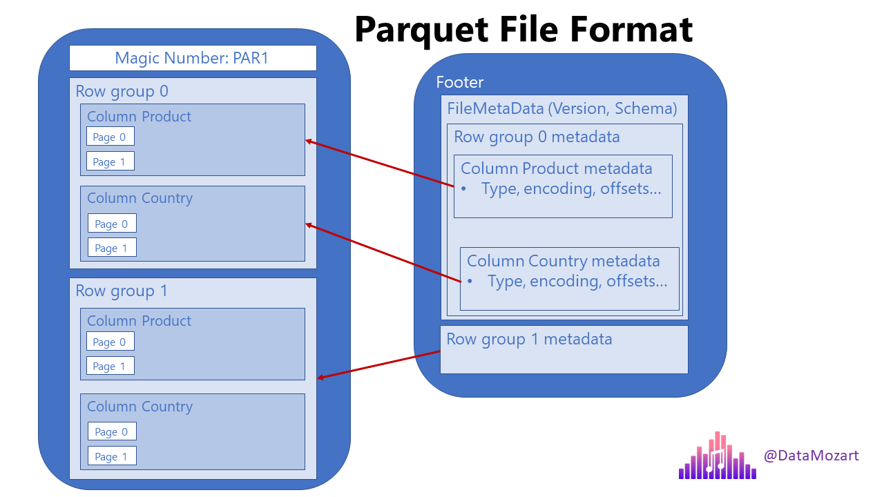
This hybrid storage model is very efficient when queries select specific columns and filter rows at the same time; a common pattern in data science: compute the correlation between homeValue and NumberOfRooms for homes where ZipCode = 24060.
Parquet stores metadata about the row chunks to speed access to rows, the metadata tells the reader which row chunks to skip. Also, a single write to the Parquet format can generate multiple .parquet files. The total data is divided into multiple files collected within a folder. Like NoSQL and NewSQL databases, data are partitioned, but since Parquet is a file format and not a database engine, the partitioning results in multiple files. This is advantageous for parallel processing frameworks like Spark that can work on multiple partitions (files) concurrently.
Parquet uses several compression techniques to reduce the size of the files such as run-length encoding, dictionary encoding, Snappy, GZip, LZO, LZ4, ZSTD. Because of columnar storage, compression methods can be specified on a per-column basis; Parquet files compress much more than text-oriented CSV files.
Because of its complex file structure, Parquet files are relatively slow to write. The file format is optimized for the WORM paradigm: write-once, read many times.
| CSV | JSON | Parquet | |
|---|---|---|---|
| Columnar | No | No | Yes |
| Compression | Yes | Yes | Yes |
| Human Readable | Yes | Yes | No |
| Nestable | No | Yes | Yes |
| Complex Data Structures | No | Yes | Yes |
| Named Columns | Yes, if in header | Based on scan | Yes, metadata |
| Data Types | Based on scan | Based on scan | Yes, metadata |
Apache ORC
The Apache ORC (Optimized Row Columnar) open-source file format, like the Parquet file format, was originally associated with the Hadoop Big Data ecosystem. ORC files have a purely columnar storage format unlike the row-group/column chunk hybrid storage in Parquet files.
ORC files are split into individual files that contain a collection of records; with columnar storage within the file. ORC files are organized into stripes, a stripe combines an index, the data in columnar form, and a footer with metadata. Stripes are essential to ORC files; they are treated independently of each other to support parallel data processing.
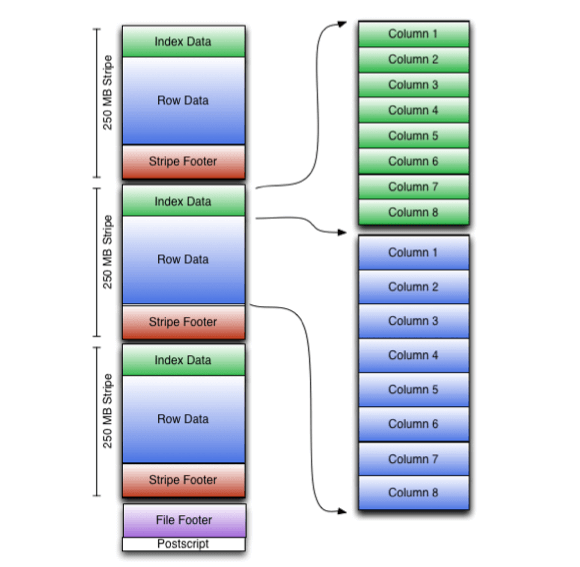
A stripe is by default 64 MB in size and ORC files can have multiple stripes. The file type was designed to store large amounts of data.
The ORC format was optimized for Hive, the data warehouse in the Hadoop ecosystem. For example, Hive and ORC together support ACID transactions on top of Hadoop. You will find that outside of Hadoop, support for ORC files is not as generous as for Parquet files. For example, you can read a multi-file Parquet file with pandas in a single line of code. To read multi-file ORC files you need to append the results of reading the individual files. The pandas functions read_orc() and to_orc() to read and write ORC files are not supported on Windows.
Apache Avro
Apache Avro is an open-source, row-based, schema-based, file format. It is often used in conjunction with the streaming platform Apache Kafka, but Avro files are useful for batch processing as well. The storage format in Avro files is mixed in that the schema information is stored in JSON format while the data is stored in binary form. The schema is thus human readable.
Like the Parquet format, Avro files are self-describing, the information to access to deserialize the records is stored in the file itself. Avro files can be compressed but they do not compress as well as column stores. Heterogeneous data types within a row do not compress as well as homogeneous data within a column. Furthermore, column-oriented storage can choose optimal compression algorithms based on the data type of a column whereas row-oriented storage uses the same compression algorithm across all data types.
Like other row stores, Avro files are great for applications that write more than they read; the opposite of column stores.
The Apache Arrow Project
If you work with large data sets, if you perform data analytics, if you process batch and streaming data, if you want to perform in-memory analytics and query processing, then you should pay attention to Apache Arrow. This is an open-source development platform for in-memory analytics that supports many programming environments, including R and Python, the primary languages for data science.
Main contributors to the Python pandas project are also involved with Arrow, so there is a lot of portability between Arrow tables and pandas DataFrames. The pyarrow package is the backend for some of the read and write functions in pandas that handle Big Data formats such as Parquet and ORC.
Newer releases of pandas are leaning more on pyarrow, e.g., pandas 2.0.
Spreadsheets
Microsoft Excel is one of the most common formats to store data. Why are we discussing it here, after all the other file formats? Like CSV files, Excel files are ubiquitous and a horrific format to store data for analytics. That applies generally to all spreadsheet formats. Do not use spreadsheets for analytic data! There be dragons!
We like rectangular (tabular) layouts in rows and columns: every row is an observation, every column is a variable. While spreadsheets appear to be organized this way, there are many ways in which the basic tabular layout can be messed with:
- Cells can refer to other cells on the same or on another sheet.
- Cells can contain data, figures, calculations, text, etc.
- Cells can be merged
One of the most problematic features of spreadsheets is how easily the data can be modified—accidentally. How many times have you been in a spreadsheet, typed something, and wondered where the input went and whether contents of a cell were changed?
This is another great question to ask a potential employer when you interview: “What data formats and/or databases are you using for analytic data?” If the answer is “We email xlsx files around once a week” run; run like it is the plague. If the answer is “The primary data is stored in Parquet files in S3 buckets”, reply “Tell me more!”
13.2 Databases
According to Wikipedia, a database is an “organized collection of data stored and accessed electronically through the use of a database management system” (DBMS). The three elements are the data, a form of data storage, and DBMS software that allows a user to interact with the system. The terms database and DBMS are often used interchangeably.
Databases play a central role in the IT stack of an organization and choosing the wrong database for an application can have dire consequences with respect to availability, scalability, security, data quality, data validity, etc. The site DB-engines collects information about databases and ranks them by popularity based on a somewhat transparent algorithm. If you think there are a lot of data science tools to choose from, wait until you wade into the world of databases—DB-engines lists over 400.
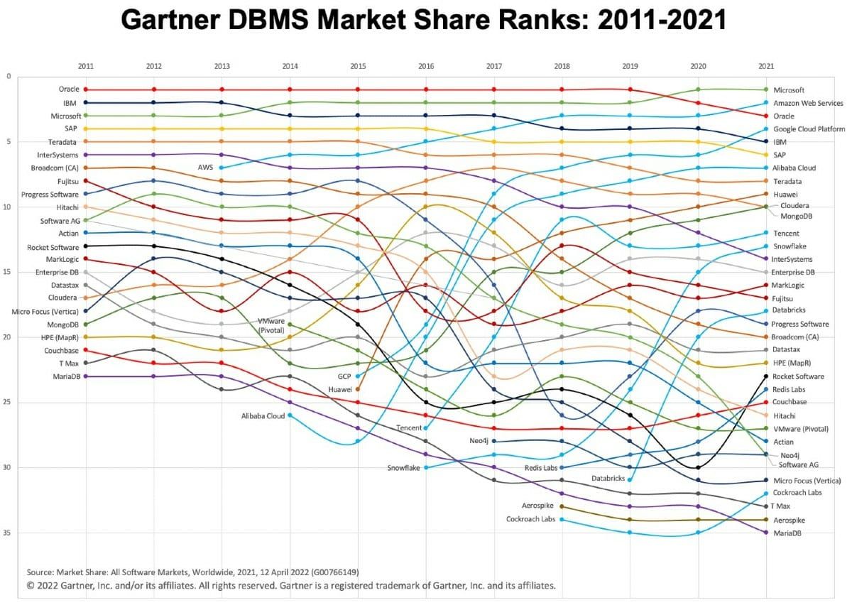
Unless you build your own tech stack, write your own application, or start your own company, you will probably not select a database. In most situations the databases have been chosen and implemented as part of the backend tech stack. Often there will be more than one, for example, MongoDB for documents, MySQL for transactions, Redshift or Spark for analytics, Redis as a memory cache—the dreaded database sprawl in organizations. Databases are part of the backend infrastructure of organizations, the part that does not change frequently. The so-called Gartner spaghetti graph in Figure 13.7 shows market share of databases between 2011 and 2021. While there is some stability near the top of the market, several items are noteworthy:
A change of guard at the top. Oracle has dominated the market for a long time and is being challenged and/or surpassed by Microsoft, Amazon Web Services, and Google Cloud Platform. The cloud providers are leading the way with compelling cloud database offerings.
Gartner depicts pure-play cloud database vendors in light blue. The spaghetti chart shows the revenue shift in databases to the cloud.
The vertical axis displays market share across all software markets. Database expenses make up about 35% of the overall software expenses. That share of the overall software market continues to increase (the chart is fanning out more toward the right).
Market share is calculated based on revenue, it does not account for free offerings, such as open-source databases.
After a peak around 2017, Hadoop-based providers of big data resources are on the decline, for example, Cloudera.
Some cloud database providers had an impressive rise since their inception, AWS since 2013, Alibaba Cloud since 2014, Google Cloud since 2015, Tencent since 2016, Snowflake since 2016.
A surprising amount of movement in a market segment that is supposed to be relatively stable. Organizations are loath to change database management systems that are key to their operations. Migrating a database that is the backbone of an essential part of the business is the last thing a CIO wants to do. Databases are not as sticky as they used to be.
It is important for anyone involved with data to understand some basics of database architectures and the strengths and weaknesses of the different database designs. A NoSQL key-value store can be a great way to work with unstructured data but can be a terrible choice for analytics compared to a relational column store. Many modern DBMS are multi-model, supporting multiple data models in a single backend, for example, key-value pairs, relational, and time-series data. There are so many databases because there are so many use cases for working with data; databases try to optimize for specific data access patterns and use cases.
Databases can be organized in several ways.
Relational and Non-relational databases
In a relational DBMS (a RDBMS) the data are organized in 2-dimensional tables of rows and columns. A database consists of a collection of named tables, each with a named collection of attributes (columns). Typically, RDBMS use SQL (Structured Query Language) to manipulate the contents of the DBMS. Each row in a table has a unique key and can be linked to rows in other tables. Relationships are logical connections between tables through keys. The structure of a table (columns, primary keys) is known as the table schema, and it is defined before the table is populated with data—this is also called a schema-on-write design (Figure 13.8).
The relational principle has dominated the world of databases since the 1980s. Seven relational databases are among the top ten databases according to DB-engines: Oracle, MySQL, Microsoft SQL Server, PostgreSQL, IBM DB2, Microsoft Access, and SQLite.
With the advent of Big Data more data was collected in ways that did not fit well with the relational paradigm: key-value pairs, documents, time series data. More fluid and dynamic relationships between data points were better captured with graph structures rather than rigid relational structures. Big Data analytics also asked for more flexibility in defining data structures on top of the raw data. The relational model was thought to be too restrictive. If the schema must be declared when the table is created and before rows are added (schema-on-write) it makes it difficult to bring new data in on the fly. Schema-on-write in relational databases requires to define the schema for the table and to structure the data based on the data. Changing the structure of the data, for example from text to numbers, requires changes to the schema and results in table copies.
Schema-on-read, on the other hand, applies structure to the data when it is read (Figure 13.9). That gives users the ability to structure the same source data differently, depending on the application. Schema-on-read led to a new class of data frameworks and databases that broke with the highly structured relational logical data model. These non-relational databases store data in key-value pairs and documents rather than tables and were also called NoSQL databases because they eschewed the structured nature of SQL-based schema-on-write. However, there is still a structuring step in non-relational databases. It just happens on demand when the data is read instead of at the beginning before the first row of data is inserted.
Non-relational databases are sometimes called schemaless databases; that goes a bit too far as some structure is needed to read the data from a key-value or document store into an application. The best translation of “NoSQL” is “not-only-SQL”, these databases still need a structured way to interact with the database.
It is easy to see how the push for more flexibility through schema-on-read goes hand in hand with the greater flexibility achieved by moving from the ETL to the ELT processing paradigm. Non-relational databases also gained popularity because they support horizontal scaling more easily than their relational counterparts. When a system scales horizontally—also called scaling out—additional machines are added to support increasing workload. Vertical scaling—also called scaling up—adds more computing resources (CPU, RAM, GPU, …) to existing machines.
You can explain the difference between the scaling models by thinking of a building with a fixed number of rooms. To increase the total number of rooms you can either add more floors (scaling up) or add more buildings (scaling out). Both types of scaling reach limits, a single building cannot be made arbitrarily tall and adding buildings consumes land. The limits for horizontal scaling are much higher than for vertical scaling.

Because non-relational systems partition data on just a primary key and do not need to maintain relationships between tables, scaling them horizontally is relatively simple. As the database grows (contains more keys) add new machines to hold the additional keys. The data can be re-partitioned by re-hashing keys across the larger cluster.
With relational systems it is necessary to maintain the relationships between the tables. When data are distributed over multiple machines, this becomes more difficult. The response of relational databases to growing data sizes has historically been to scale up. Relational databases designed with horizontal scaling in mind are referred to as NewSQL databases.
Non-relational (NoSQL) databases are categorized by their underlying data models into pure document stores, key-value stores, and graph databases—more on these designs below. NoSQL is primarily used in transactional databases for OLTP (online transactional processing) and applications where interactions with the database are limited to CRUD operations (Create, Read, Update, Delete). They are not performant for analytical jobs.
Transactional (OLTP) and Analytical (OLAP) Databases
A transactional database is a repository to record the transactions of the business, the ways in which an organization interacts with others and exchanges goods and services. Business interactions that are recorded in transactional systems are, for example, purchases, returns, debits, credits, signups, subscriptions, dividends, interest, trades, payroll, donations.
Databases that support business transactions are optimized for a high volume of concurrent write operations: adding new rows, updating rows, inserting rows. These transactions are often executed in real time, hence the name online transaction processing (OLTP).
The concept of a database transaction is different from a business transaction. A database transaction is a single logical unit of work that, if successful, changes the state of the database. It can comprise multiple database operations such as reading, writing, indexing, updating logs. A business transaction, a customer orders an item online, can be associated with one or more database transactions.
Database transactions are not just reserved for OLTP systems, although supporting transactional integrity with so-called ACID properties is a must for them. Analytic databases, graph databases, NoSQL databases typically support transactions. In relational SQL systems, look for BEGIN statements to flag the start of a transaction, the COMMIT statement to commit the results of a transaction and the ROLLBACK statement to reset the state of the database prior to the transaction.
The ACID properties refer to atomicity, consistency, isolation, and durability to ensure the integrity of the transaction.
Atomicity: all changes are performed as if they were a single operation. Either all of them are performed or none of them.
Consistency: When the transaction starts and when it finishes, the data are in a consistent state.
Isolation: intermediate states of the transaction are invisible to the rest of the system. When multiple transactions happen at the same time, it appears as if they execute serially.
Durability: After a transaction completes, changes to the data are not undone.
Take as an example the transfer of funds from one account to another. Atomicity requires that if a debit is made from one account a credit in the same amount is made to the other account. Consistency requires that the sum of the balances in the two accounts is the same at the start of the transaction and at the end. Isolation implies that a concurrent transaction sees the amount to be transferred either in the debited account or in the credited account. If a concurrent transaction would see the amount in neither account or in both accounts the database fails the isolation test. Durability means that if the database fails for some reason after the transaction completes, the changes made to the accounts will persist.
Examples of transactional (OLTP) relational databases are MySQL, PostgreSQL, Microsoft SQL Server, Oracle Database. These systems are also called Systems of Record (SoR) because they store the official records of an organization—the ground truth. While NoSQL databases can support transactions, they relax some of the criteria to support greater scalability. The According to the CAP theorem, a distributed database that partitions data across different machines cannot be fully ACID compliant and guarantee availability. When a network partition fails one must choose between availability of the system and consistency. A relaxed condition is eventual consistency, where the data achieves a consistent state sometime in the future. Eventually, all reads will return the most recently written data value. For systems of records in financial services eventual consistency is not acceptable; SoRs must be ACID compliant.
Why are these arcane details of database architecture important for a data scientist?
Database designers make tradeoffs when optimizing for a use case. You should be aware how these tradeoffs can affect data integrity if that matters for your project—it might not be an issue at all.
Using an OLTP system for analytical work is usually a bad idea. Transactional systems need to respond to frequent data updates and tend to return small record sets when queried (look up a customer, look up an account balance). The best way of storing information for this pattern is as a row-store: the data for a record is stored in a chunk of memory which makes retrieval of a record or set of record very efficient.
Row and Column Storage
Table 13.2 shows seven of the 150 observations from the famous Iris data set that is used in statistics and machine learning courses to apply regression, classification, and clustering methods. The full data set contains 50 observations for each of three Iris species: Iris setosa, Iris versicolor, and Iris virginica. Four measurements of the flowers, the length and width of the petals (the large leaves on the flowers) and the sepals (the small leaves) were taken on each plant.
| SepalLength | SepalWidth | PetalLength | PetalWidth | Species | |
|---|---|---|---|---|---|
| 5.1 | 3.5 | 1.4 | 0.2 | setosa | |
| 4.9 | 3.0 | 1.4 | 0.2 | setosa | |
| 4.7 | 3.2 | 1.3 | 0.2 | setosa | |
| 4.6 | 3.1 | 1.5 | 0.2 | setosa | |
| 5.0 | 3.6 | 1.4 | 0.2 | setosa | |
| 7.0 | 3.2 | 4.7 | 1.4 | versicolor | |
| 6.4 | 3.2 | 4.5 | 1.5 | versicolor |
Suppose we store this data in a row-store with a fixed record length. The numerical measurements can be stored in 4-byte floats. The longest string in the Species column is 10 characters long. To align the records on 4-byte boundaries for faster access, we set the record length to 4 x 4 + 12 = 28. Figure 13.11 shows the first row of data set is laid out across 28 bytes.

Suppose that the data is stored in one big chunk of memory, each row starts 28 bytes after the previous row.

Looking up rows is extremely fast. To read the data for the third observation jump to byte 56 and read the next 28 bytes. Adding new records in row-oriented storage is also fast: allocate a new chunk of 28 bytes and fill in the fields. However, if we want to perform an analytic operation such as computing the average petal length, we must jump through the memory and grab values at position 8, 8 + 28, 8 + 56, …., 8 + 150 x 28. That is very inefficient, especially when tables have many columns and records are long.
To support fast analytic processing, analytical databases are optimized for an access pattern where data is mostly read and infrequently written (changed). The ease of appending or looking up entire rows is then not as important as the efficiency of accessing memory for a column. Analytical queries are deep in that they process information from many records in the table—rather than looking up records—and they can return large result sets. Also, analytical queries tend to operate on a small subset of the columns of a table rather than all the columns.
The best-performing format for storing information for this workload is a column-store: each column in the table is stored in one or more chunks of memory.
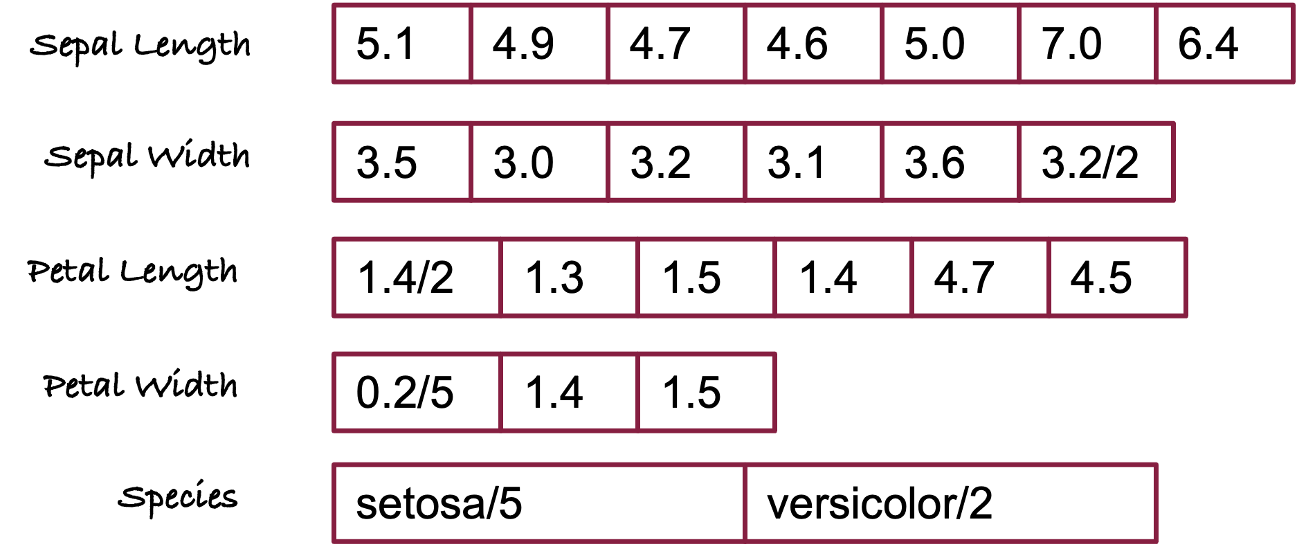
Figure 13.13 shows the five columns in the Iris data set in column store format. Computing the average of, say, sepal length, can now be done efficiently by scanning the memory for that column. The data for the other columns does not have to be loaded into memory for this operation.
Columnar storage has other advantages for analytic databases: the data types are homogeneous within a block of memory (all characters, all integers, all floats, etc.) and compress well. Except for sepal length, all columns have repeated values. These can be stored along with an integer that counts the number of times a value appears. This simple technique—called run-length encoding—can greatly reduce the storage requirements when the data are ordered and have repeat values.
The following is a non-exhaustive list of analytic databases that use columnar storage:
- Amazon Redshift
- Google BigQuery
- Azure Cosmos DB
- DuckDB
- Vertica
- ScyllaDB
- DataStax
- ClickHouse
- Apache Druid
- Apache Cassandra
- Apache HBase
Hybrid (HTAP) Databases
Some databases combine row-oriented storage with column-oriented storage in the same database engine; this paradigm is called hybrid transactional-analytical processing (HTAP). The idea behind HTAP databases is that you do not need two separate databases, one for transactional workloads and one for analytical workloads. The ability to perform both workloads efficiently in the same database reduces data movement and data duplication between databases. This reduces the dreaded database sprawl in organizations. The term HTAP was coined by industry analyst firm Gartner. Forrester, Gartner’s competitor, refers to this processing paradigm as translytical.
Another motivation of HTAP databases is that transactional systems, where information about the business is recorded in real time, also need support for real-time analytics to produce insights “in the moment”. Transactional systems are becoming more analytical, the results and side effects of algorithms triggered by a transaction can be the most important piece of information of the transaction.
Ride Share Booking
Suppose you land at the San Francisco airport and use your favorite ride share app to book a ride into the city. This starts a transaction with the ride share company. The data recorded as part of the transaction includes customer information, origin and destination of the trip, time of day, etc. In real-time, as the transaction occurs, the backend of the app calculates the price for the ride based on location, traffic density, ride demand, available drivers, vehicle type, etc.
This is an analytical operation that invokes a price-optimization algorithm. Based on the real-time prices offered to you in the app, you choose the preferred ride. The optimized price is recorded as part of the transaction.
The following are examples of HTAP databases:
- PingCAP
- Aerospike
- SingleStoreDB (formerly MemSQL)
- InterSystems
- Oracle Exadata
- Splice Machine
- GridGrain
- Redis Lab
- SAP/HANA
- VoltDB
- Snowflake (since the addition of Unistore in 2022)
- Greenplum
NewSQL Databases
As a broad generalization we can state that non-relational NoSQL databases sacrifice consistency for horizontal scalability and that traditional relational SQL databases are ACID compliant but do not scale well horizontally, they are designed for scale-up.
NewSQL databases try to bridge this gap, providing horizontal scalability and transactional integrity (ACID compliance). There are variations in the types of transactional guarantees they provide, so it is a good idea to read the fine print. For example, a transaction might be defined by a single read or write to the database rather than the operations wrapped in a BEGIN—COMMIT block.
NewSQL databases tend to have in common:
Data partitioning: the data are divided into partitions (also called shards). Partitions can reside on different machines.
Horizontal scaling: because of sharding, the database can accommodate an increase in size by adding more machines.
Replication: The data appears in the database more than once. Replicates can be stored on the same or different machines, availability zones or regions. For example, one machine can serve as the primary node for some partitions and as a backup node for replicates of other partitions. This provides failure resilience and the ability to recover the database from disasters.
Concurrency control: to maintain data integrity under concurrent transactions.
Failure resilience: the databases recover to a previous consistent state when machines fail or the database crashes.
The following are examples of NewSQL databases:
- CockroachDB
- VoltDB
- SingleStoreDB
- ClustrixDB
- Pivotal Gemfire
- NuoDB
Non-relational Database Designs
Because non-relational (NoSQL) databases have become popular and play an important role in data analytics, we want to spend a few moments on their principal architecture. The primary designs for NoSQL databases are
- Key-value stores
- Document stores
- Graph databases
Non-relational databases can be multi-model and support more than one design. Many graph databases on the DB-Engines list support document store, key-value, and graph models.
Key-value stores
In a key-value store, every item in the database has only two fields, a key and a value. For example, the key could be a product number and the value could be a product name. This seems restrictive, but the value does not have to be a scalar, it can be, for example, a JSON documents with subfields.
| Key | Value2 |
|---|---|
| “username” | “oschabenberger” |
| “account type” | “personal” |
| 345625 | { name: “MacBook Pro 16”, processor: “M2”, memory: 32GB” } |
| 165437 | { name: “Paper towel”, available: true, discount: 10%” } |
To achieve horizontal scaling (scaling out) of key-value stores, the data are partitioned across multiple machines based on a hash table. For a database with \(n\) machines the hash is essentially a mapping from the key to the integers from 0 to \(n-1\) that determines on which machine a particular key is kept. As the database grows (more keys added) more machines can be easily added. Such scaling out is more difficult in relational systems where the relationships between the tables must be maintained as the data is distributed over more machines. That is why not building tables on relations supports horizontal scaling. While documents are grouped into collections (the NoSQL version of a table), there is no association or relationship between one document or any other. The relative ease to scale horizontally is one reason why non-relational databases became so popular for handling large and growing databases.
Disadvantages of key-value stores are also apparent: items can only be looked up by their (primary) key. Queries that filter on other attributes are less efficient than in relational systems: what is the average order amount of customers who ordered fewer than 5 items in the last 12 month? It is difficult to join data based on keys. They are not as performant for analytical work as relational systems, especially those with columnar storage layers. A good application for key-value stores are CRUD applications where items are merely created, read, updated, and deleted.
Document stores
A document store extends the simple design of the key-value store. The value is now stored as a document-oriented set of fields in JSON, XML, YAML, BSON, or similar format. While the data in a key-value store is transparent to the application but deliberately opaque to the database, in a document store the values are transparent to the database. This enables more complex queries than just using the primary key, the fields in the document can be queried.
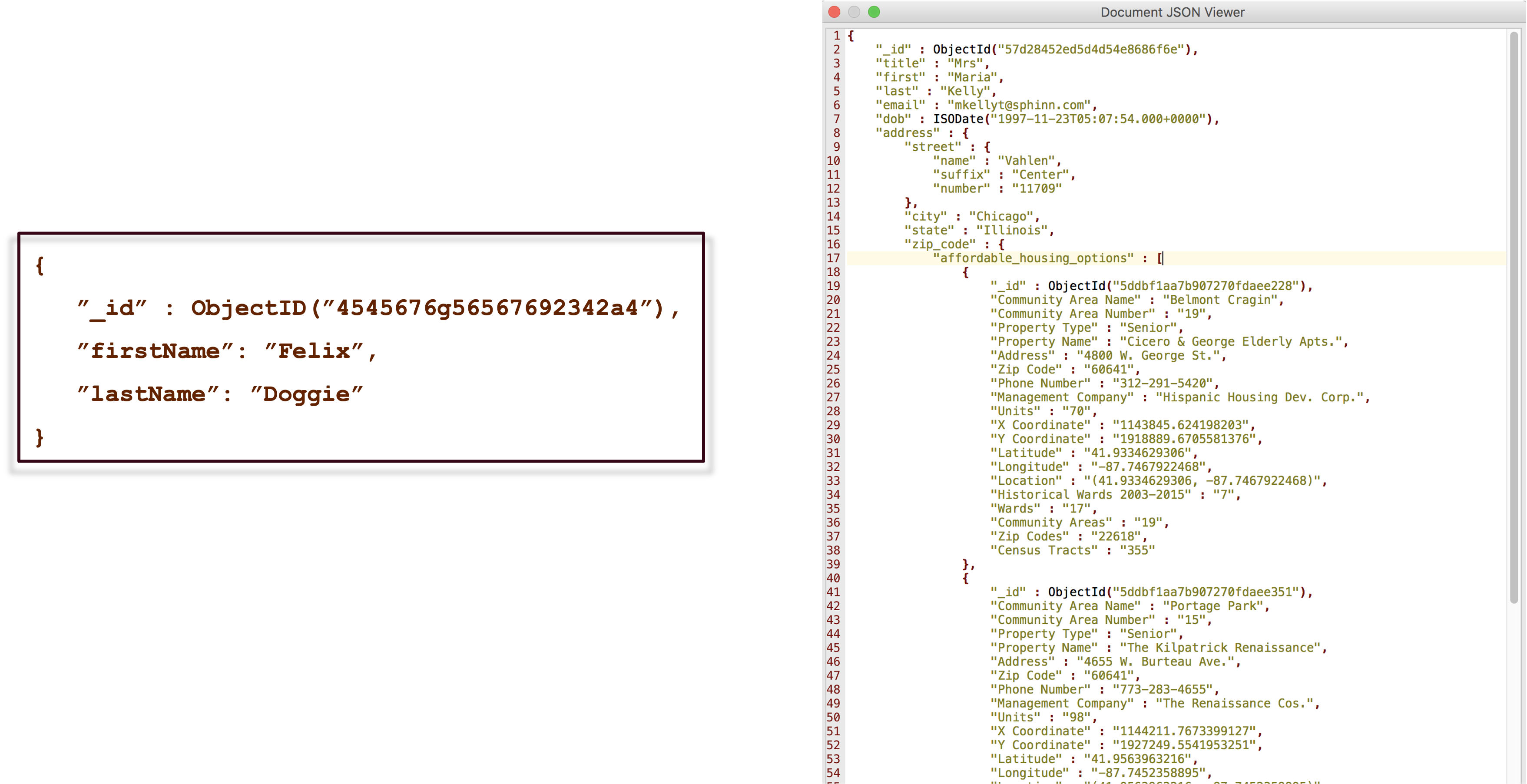
The fields of the documents do not have to be identical across records in the database. For example, documents containing customer names have a field for a middle initial only if the individual has a middle initial. Documents do not contain empty fields. In contrast, a relational system that stores a middle initial will have this field for all records and NULL values are used to signal an empty field when a middle initial is missing.
Like key-value stores, document databases are great for CRUD applications, but do not perform well for analytical queries and cannot represent relationships and associations. Each document exists as an independent unit unrelated to other documents.
Graph databases
In graph databases relationships are a first-class citizen. The relationships are not expressed through keys in tables, but through edges that connect nodes (vertices). Nodes are the entities of interest in the database such as people, products, cities. Nodes have attributes (called properties) stored as key-value pairs or documents (Figure 13.15).
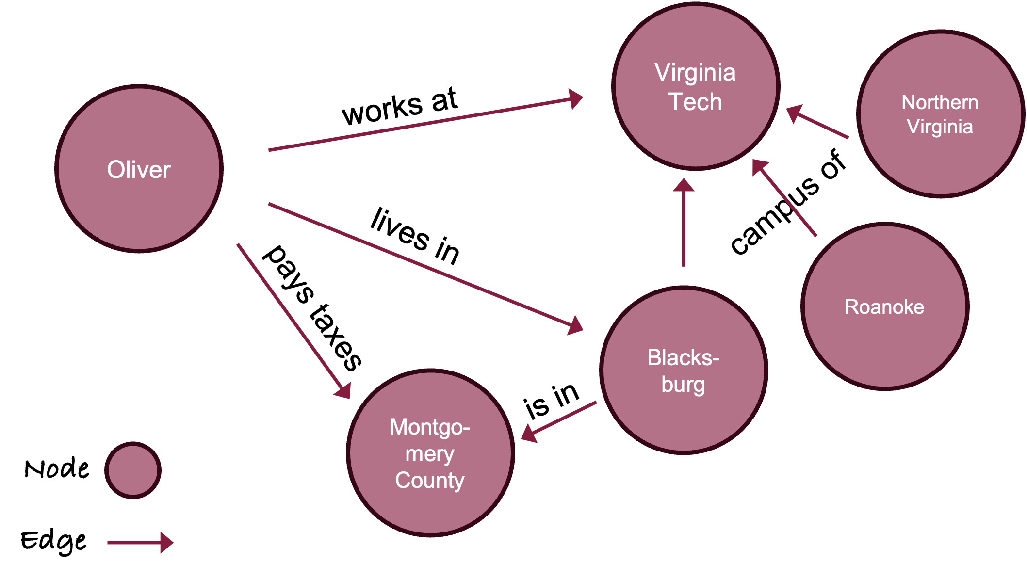
Because of this storage model graph databases are considered NoSQL databases. Labeling them as non-relational databases is only correct with respect to the traditional table-based relational systems. Relationships are a central property of graph databases, and they are more flexible and dynamic compared to RDBMS. Relationships emerge as patterns through the connections of the nodes rather than predefined elements of the database.
This list shows the DB-Engines ranking of graph database systems. Note that many of them also support key-value or document stores.
13.3 Cloud Databases
According to statista, the share of corporate data stored in the cloud has increased from 30% in 2015 to 60% in 2022. The total addressable market (TAM) in cloud computing is estimated to exceed $200 billion per year and is growing by double digits.
The market for storing data in the cloud as files, blocks, or generic objects is a staggering $78 billions of that TAM (2022) and the market for cloud databases is $21 billions in 2023. The cumulative aggregate growth rate (CAGR) for cloud storage and cloud databases is 18% and 22%, respectively. What do we take away from these numbers?
Cloud computing is one of the most fundamental revolutions in computing in the last 20 years.
Half of the addressable market is in storing data, either in databases or in some other form of cloud storage (files, blocks, objects). Getting your data into their cloud is a key element in the business model of the cloud service providers (CSP). Data has gravity and its “gravitational constant” seems to increase as it comes to rest in a cloud data center.
The economics of inexpensive cloud storage will continue to erode Big Data storage systems like Hadoop (HDFS).
Transactional and operational systems are unlikely to be supported by object storage, while it is least expensive it is also least performant. That is where databases optimized for transactions and/or analytic of cloud data come in.
A database is said to be cloud-ready if it can be run on cloud infrastructure. That is true for most databases. It is said to be cloud-native if the database was designed for the cloud and takes advantage of the full functionality of the cloud, for example, horizontal scaling (scale-out) with increased workload, separation of storage and compute, container deployment and Kubernetes orchestration, multi-tenancy, disaster recovery, bottomless storage.
Among cloud databases we can broadly distinguish three service models according to who takes on the responsibility for maintaining the infrastructure, the database instance, and the access to the database: self-managed databases, managed services (DBaaS), and serverless databases.
Self-managed
A self-managed cloud database is not much different from a database installed on premises, except that it uses cloud infrastructure. As the name suggests, you are responsible for administering and maintaining all aspects of the deployment. The CSP will provide the infrastructure and make sure that it is operational, but you must make sure that the database running on the platform is operational, updated. You can install any database of your choice, including not cloud-native databases.
Some cloud-native databases offer a self-managed option, but a managed service or serverless offering is more typical when databases were designed specifically for the cloud.
Managed Service
Also known as database-as-a-service (DBaaS), this deployment methodology is a special case of software as a service, where the software managed on behalf of the user is a database system. In exchange for a subscription, the service provider handles the management of the database, including provisioning, support, and maintenance. The service provider chooses the hardware instances on which the database runs, frequently using shared resources for multiple databases and customers.
Here are examples of relational and NoSQL databases offered as a managed service:
Relational
- SingleStoreDB
- CockroachDB
- Amazon RDS (Relational Database Service)
- Azure SQL
- MotherDuck (SaaS for DuckDB)
- Azure DB for MySQL, PostgreSQL, …
- Google BigQuery
- Google Spanner
- Oracle Database
NoSQL
Cloud service providers have been pushing non-relational systems because horizontal scaling fits well with their business model: adding cloud infrastructure drives revenue for the cloud provider.
Serverless Systems
We need to explain what we mean by “serverless computing” because all code executes on a computer (a server) somewhere. Serverless computing does not do away with servers. It eliminates for software developers the particulars of worrying about which servers their code runs on. This sounds a bit like the SaaS model, but there are important distinctions between a serverless and a serverful (e.g., SaaS) system:
In serverless computing you execute code without managing resource allocation. You provide a piece of code to the CSP, and the cloud automatically provisions the resources necessary to execute the code.
n serverless computing you pay for the time the code is executing, not for the resources reserved to (eventually) execute the code. The provider of a serverless service is then encouraged to scale back computing resources as much as possible when not in use (known as scale-to-zero).
Serverless computing can be seen as the latest form of virtualization in computing. The user writes a cloud function and ties it to a trigger that runs the function, for example, when a customer opens an online shopping cart. The serverless system then takes care of everything else such as instance selection, logging, scaling, security, etc.
Not all applications are suitable for serverless computing and for some time databases where thought to be among the backend services that do not fit with the serverless paradigm (see, for example, this view from Berkeley):
Serverless computing is essentially stateless computing: the state necessary to execute code is either sent over an API along with the request or is stored somewhere server-side between function calls.
Databases have a lot of state, such as connection protocols, metadata, access controls, schemas, etc.
Databases often use connection-based protocols which assume a stable connection over a port between a host and a client. That conflicts with the design of serverless systems.
Databases have a cold-start problem. A cold start is the time required to instantiate an environment and to get things up and running when a function is called for the first time. In a serverful environment you encounter a cold start only once at the beginning. In a serverless environment cold starts happen the first time you invoke a service and every time the system has scaled back. For example, if the serverless database quiesces after 5 minutes of inactivity and you submit queries every 10 minutes then every query must go through an instantiation of the database environment, including loading the data.
Despite these challenges there has been a lot of progress in serverless database systems in recent years. Here is an incomplete list of relational and NoSQL serverless cloud databases. Notice that the list contains databases listed earlier; some providers make DBaaS and serverless options available:
Relational
- MotherDuck (collaborative serverless platform built on DuckDB)
- Neon Serverless Postgres
- PlanetScale DB (Serverless MySQL)
- CockroachDB Serverless
- Amazon Aurora Serverless
NoSQL
A special shout-out to DuckDB, a lightweight, embedded, analytical RDBMS that runs inside a host process, for example, inside a Python or R session. DuckDB integrates very well with other systems; it makes working with a relational system from Python or R very easy. MotherDuck is a serverless platform and cloud database built on DuckDB. The integration between the two makes working with databases locally and in the cloud particularly easy. And since DuckDB is optimized for analytic workloads, DuckDB & MotherDuck are great choices for data scientists. We will see more of DuckDB in the chapters that follow.