29  Bias and Harm in Algorithms

29.1 Are Data Biased?

The previous section presented examples where things went wrong, where algorithms had unintended consequences and side effects. It is easy to say that the data is biased and thus the fault lies with the data used in training models. The data can be a major source of problems in data analytics. But the answer cannot be as simple as saying “garbage—in—garbage—out”.

Training models on data that are not representative of the situation to which the model will be applied is just one possible form of bias, called representation bias. It can occur even if the data was collected perfectly, measured without error, sampled adequately—for a different purpose than it is now used. This is not unlike our statistical understanding of bias, as the (average) difference between an estimator and its target. A perfectly qualified estimator can be biased for one target and unbiased for another target. The sample mean \(\overline{Y}\) of a random sample is an unbiased estimator of the mean \(\text{E}[Y] = \mu\) of the sampled population and is a biased estimator of the median of the population unless the distribution of \(Y\) is symmetric (mean and median are then identical). Context matters.

Rather than taking a 30,000-foot view that “data are biased” or “data can be biased” and harm of data-dependent models is a possible consequence, it is worthwhile to drill deeper and ask what types of biases exist and how unintended consequences and harm flows from the way in which we build, test, and deploy models. Data can be biased. We need to ask in what way bias can be introduced into data, through data, and through processing data. Without this understanding we cannot apply remedies.

Algorithms are normally not purposefully built to be unfair or cause harm. Instead, they are the result of processes that lead to algorithms that make unfair or harmful decisions. So how does it happen that an algorithm in Austria determines that women have lower employability than men if all other characteristics are equal? How is it possible that female job seekers are less likely to see advertisements on Google for high-paying jobs than their male counterparts? We know that the algorithm is unfair because we can test it. That is exactly what researchers from Carnegie Mellon did; they put the advertisement algorithm through the ringer with a designed experiment. As reported by the Guardian:

One experiment showed that Google displayed adverts for a career coaching service for “$200k+” executive jobs 1,852 times to the male group and only 318 times to the female group. Another experiment, in July 2014, showed a similar trend but was not statistically significant.

In the excellent paper “A Framework for Understanding Sources of Harm throughout the Machine Learning Life Cycle”, on which this discussion is partly based, Suresh and Guttag (2021) give the following example where the same intervention to correct bias works in one case and fails in another.

Example: Sample More Women

The goal is to build a model to predict the risk of a heart attack. A researcher trains a model on medical records from prior patients at a hospital and observes that the false negative rate of the trained model is higher for women than for men. Assuming that the reason for the poorer predictive performance is a lack of data on women in the records, the researcher adds more data on women who suffered heart attacks. The re-trained model shows improved performance in predicting heart attacks in women.

In another application, a hiring model is developed to determine suitability of candidates based on their resume, augmented by candidate ratings supplied by human evaluators. It is observed that the model predicts women to be less likely as suitable candidates compared to men. To correct this shortcoming, more data is collected on women, but the model does not improve. In both scenarios the model builders recognized a deficiency in the model and tried to correct it—that is ethical behavior.

But the same intervention, collecting more data on the group for which the model performed poorly, was successful in one instance and pointless in the other. The reason is that the model deficiency is due to different sources of bias. In the medical example, the training data under-represented women, there was not enough information about women in the data to create a model that was as accurate for that group as it was for the group more heavily represented in the data—men.

Modifying the sampling process changed the distribution of genders in the training data. In the hiring example, the bias is not introduced through the representativeness of the sample, but through the human-assigned rating. When the human assessment of candidate suitability disadvantages women over men, adding more data will not correct the model.

29.2 Seven (Eight) Sources of Harm

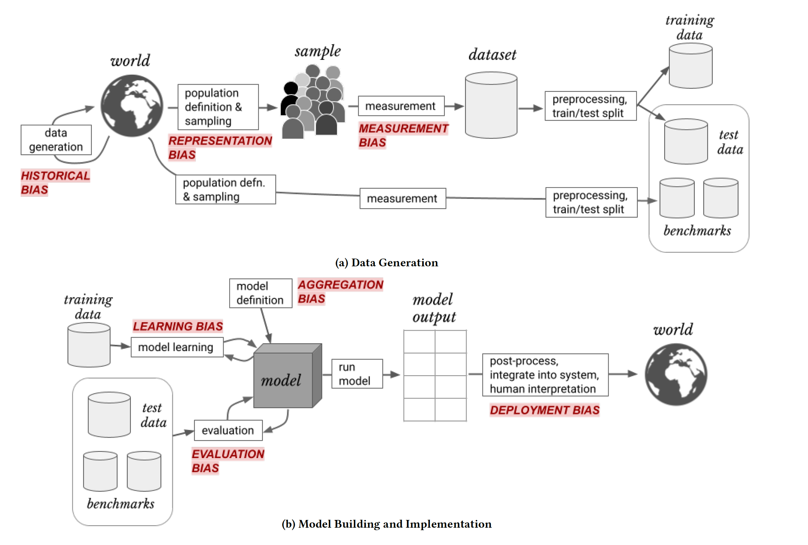
Suresh and Guttag (2021) describe seven distinct sources of bias and associate them with steps in the modeling cycle, from data preparation to model deployment.

Figure 29.1: The seven sources of harm in machine learning models (Suresh and Guttag 2021).

Historical Bias

Models do not extrapolate what they learned from the training data to situations that do not reflect the training data. They can create associations only from what is in the training data: the past is prologue.

A system that reflects accurately how the world is or was can inflict harm, either by unfairly withholding resources (allocation harm) or by perpetuating stereotypes (representational harm).

Historical bias, also called pre-existing bias, is rooted in social institutions, practices and attitudes that are reflected in training data. Baking these into the algorithm reinforces and materializes the bias. In the example of the Austrian employability algorithm, the data reflected an accurate representation of a discriminatory labor market, women, especially women with children, are less likely to be found in high-paying jobs. The algorithm trained on this data assigned a lower employability score to women.

If you train a model on data from textbooks, then it is more likely to identify engineers as men than as women, since that profession is historically more likely to be depicted by men. Word embeddings are numerical representations of text data used to train language models. Any stereotypes in the source texts on which the embeddings are based will live on in the models developed based on the embeddings.

The historical bias might not be evident right away. It can rear its ugly side when the model is applied in an unforeseen way. Google Translate got into trouble when documents were translated from Hungarian into English. Hungarian is a gender-neutral language, so the algorithm had to apply pronouns in the English translation. From the article on DailyMail.com:

‘She’ was placed before domestic chores such as cleaning and sewing, while ‘he’ was used for intellectual pursuits such as being a politician or a professor.

‘He teaches. She cooks. He’s researching. She is raising a child. He plays music. She’s a cleaner. He is a politician. He makes a lot of money. She is baking a cake. He’s a professor. She’s an assistant.’

The researcher who found the issue blamed Google. Google blamed the algorithm on society: the algorithm inadvertently replicated gender biases that exist in the information it scraped from the internet.

How can we fix this type of bias?

• Change the data. One could revisit the training data in the translation example and change gender pronouns to achieve better balance across attributes. The trained algorithm then would hopefully reflect that balance. Modifying data is considered unethical. There be dragons! What proportion of female pronouns should be used for, say, a profession. The currently prevailing proportion or a desired future state? In Hungary or the U.S? Who decides what that is?

• Use different data. Finding a data source that does not have historical bias baked into it sounds good but might not be possible.

• Adjust the model. Corrections can be made to the inner workings of the model. For example, instead of using gendered pronouns the translation can use gender-neutral language: “they cook, they teach”. Alternatively, the gender pronouns in the translation can be chosen randomly.

Representation Bias

Representation bias bias occurs because of a mismatch between sample, target, and application population. The target population is the universe we have in mind in developing an algorithm. The sample population is the population represented by the training data. The application population is the universe to which the model is applied. It is easy to create mismatches.

A model developed for house values in Boston probably does not apply in Chicago without re-training on data from Chicago. The target population (Boston) and application population (Chicago) are mismatched.

Sampling bias—also called selection bias—is a form of representation bias where the sampling method is defective and does not represent the target population. A random sample is always representative of the target population but there are many ways in which the training data can deviate from the properties of a random sample from the target population:

• Available data can misrepresent the target population, for example, if medical data is only available for individuals having a condition.

• Random sampling that does not reflect the distribution of groups in the target population, for example, drawing random samples from lists of users (website, mobile phone, phone book, tax records) does not accurately represent the overall population (over-/under-coverage).

• Missing values processes that are related to the objective of the study. When recipients in a mental health survey are less likely to respond because of their mental health status, the sample of survey responses is biased (non-response bias).

• Self-selection: participants who exercise control over their inclusion in a study can bias the data. Folks calling into radio shows or participating in online polls are particularly motivated by issues and their responses overestimate strong opinions in the population.

• Survivorship bias can occur when the sample focuses on those meeting a selection criterion. For example, studying current companies does not reflect companies that have previously failed.

• Drop-out: subjects drop out of a long-term study for reasons related to the objective of the study. Losing study participants in a longitudinal health study that move out of the area because of a new job probably does not bias the data. Losing study participants because of deteriorating health might bias the data.

Example: Literary Digest Poll

A famous example of sampling bias because of under-coverage and non-response bias was the 1936 poll by the Literary Digest magazine to predict the outcome of the presidential race between incumbent Democratic candidate Franklin D. Roosevelt and Republican candidate Alf Landon. The magazine sampled voters based on its own subscribers, phonebooks and car registration data and predicted that Alf Landon would win the election.

Instead, Franklin D. Roosevelt defeated Landon in a landslide. Although it had sampled millions of voters, the magazine’s prediction was way off, by more than 19%. The embarrassment contributed to the magazine’s demise by 1938.

Sampling bias due to an inappropriate sampling frame was one factor for the imprecise survey. Subscribers to Literary Digest, phone users and automobile owners were on average wealthier than the average American. Their responses over-estimated the proportion of Republican voters. The second, and primary source of bias was non-response bias: those who disliked Roosevelt were more likely to respond in favor of Landon.

In an earlier chapter we mentioned ImageNet, a large database of images used in computer vision challenges and to benchmark object classification algorithms. ImageNet does not represent a random sample of all images that could be taken. Almost half of its images originate in the U.S., only 1—2% of the images come from China and India. A computer vision model trained on ImageNet data is expected to perform worse classifying objects from images from those geographic areas.

This is a special kind of bias. Groups that occur in the data less frequently are predicted with less accuracy, simply because there are fewer training samples in those groups compared to others. In the ImageNet example this is due to the way the data are collected from the internet. If a population is properly sampled randomly, minorities will appear less frequently in the sample than majorities. When model performance is analyzed stratified by groups, the model will be less accurate (have a larger prediction error or mis-classification rate) for groups that contributed fewer observations. Differentiated levels of accuracy are unfair and potentially harmful.

The cause of representation bias might not be immediately obvious, while its presence can be very obvious in the results.

Example: “Delving” into ChatGPT

Jeremy Nguyen asked on X (Twitter) why there was such an increase in the recent use of “delve” in medical papers and presented Figure 29.2 as evidence. The tweet appeared in March 2024, so we still had a long way to go in that year to grow the bar on the right.

Figure 29.2: Use of “delve” in papers on PubMed. Source:JeremyNguyenPhD on X

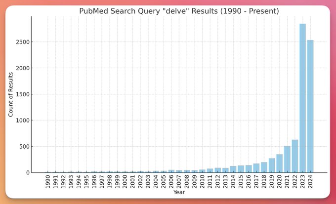
Use of “delve” has been on the increase for some time, but in 2023 it took off dramatically. Do medical papers just do more delving since then? It has been noted that ChatGPT responses seem to use certain words more frequently than the internet at large. Examples are “delve”, “explore”, “tapestry”, “testament” and “leverage”. Frequently enough to be seen as a giveaway that text was generated by GPT. GPT 3.5 was released in late 2022 and 2023 is the first full year the world enjoyed ChatGPT. Is Figure 29.2 evidence that (many) medical papers are now being written—or at least augmented—with the help of ChatGPT?

How is it possible that GPT, which is trained on a massive corpus of text found on the internet, has such an affinity for “delve” and uses it more frequently than would be consistent with the training data? The reason is a special form of representation bias. ChatGPT is a question-answer application built on top of the foundation large-language model GPT. The ChatGPT training uses a form of reinforcement learning, called reinforcement learning with human feedback (RLFH). That is a fancy way of saying that in order to perform reinforcement learning, the algorithm needs a reward function with which to rate competing actions–that is, competing responses to the prompt. Scoring the quality of a textual response is difficult and this is where human evaluators come in. The human evaluation can alter or correct an initial response from the AI to create a response with a higher reward score. When this altered response is fed back into the algorithm, the model will eventually learn to respond to maximize the reward, and respond in a way similar to the human evaluator.

This is the first part of the story. The second part of the story is that human evaluation and feedback in training LLMs is time consuming and costly. That is why tech companies outsource this work to places where anglophonic knowledge workers are cheap. As the Guardian points out in this article, “delve” is much more frequent in business English in Nigeria than in the U.S. or the U.K. Outsourcing the task to provide human feedback to Nigeria creates a feedback loop that makes ChatGPT write more African English than its original training data.

Measurement Bias

Measurement bias—also called detection bias or information bias—is due to systematic errors in the process of data collection. Random data measurement errors do not contribute to measurement bias, they cause greater variability in the data. A scale that is not properly calibrated, on the other hand, will give systematically incorrect readings of weight—that is a biased measurement.

Incorrect instruments are a source of this bias and insufficient accuracy or limitations of the instruments. Measuring distance that exceed 10 feet with a 10-foot tape measure causes observations to be censored. The true distance is larger than 10 feet, but we do not know the exact value. The accuracy of instruments can vary with its range; being most accurate in the mid-range and less accurate above or below.

Bias in measurements applies to qualitative variables as well, for example, when survey interviewers ask participants to rate their satisfaction for the wrong timeframe.

These sources of measurement bias are obvious. Suresh and Guttag also discuss a type of measurement bias that could be called proxy bias. The target variable of interest is often not directly observable. Instead, we use proxies to operationalize the concept of interest. Creditworthiness, for example, is not directly observable, and we use credit scores as the proxy. To model student success, we need to define what we mean by that. The choice of proxy affects the quality of the inference. An oversimplification such as GPA can bias the results because it does not apply to all students, does not capture learning outside of the classroom, does not capture skills not assessed as grades, etc.

While the concept of interest is consistent across groups, e.g., has a disease, the technique for measuring its proxy, the diagnosis, can vary among groups. Regional or cultural differences lead to different interpretations of the same context when annotating images. The same 5-point rating scale is used differently depending on someone’s interpretation of the categories. Does the “best” category mean “best in my experience so far” or “the best one could ever hope for”?

In the COMPAS system for predicting recidivism discussed previously, variables like arrested and re-arrested are proxies for criminality. Measurement bias is introduced when certain communities are policed more intensely than others. If the extent to which a higher number of arrests reflects a higher policing intensity is not accounted for, the analysis will be biased and disadvantage the community where policing is higher.

Aggregation Bias

Aggregation bias occurs when data are grouped or aggregated in a way that ignores or obfuscates important subsets of the data. Trends and associations that we see in aggregated data are not necessarily present in the non-aggregated data. Similarly, trends and associations in non-aggregated data can be missed in aggregated data. For example, working with data at an annual level hides seasonal trends. This can be desirable. It can also lead to bad decisions by not accounting for systematic variation at a smaller level.

Confusing the units of inference with the units of analysis is known as an ecological fallacy: to assume that what is true for a population is also true for the individual members of the population. One commits an ecological fallacy by concluding that individuals from families in poverty perform less well in school by studying the correlation between average poverty level in schools and school test averages. The analysis is based on aggregates at the school level, an association at that level does not imply an association at the individual level. A proper analysis takes a multi-level approach that models effects at the student, classroom, and school level.

Learning Bias

This type of bias occurs when the process of training the model introduces bias by emphasizing some criteria more than others. For example, classification models are often trained to minimize the mis-classification rate (maximize the accuracy) on a test data set. Models with a high accuracy are not guaranteed to have a high true positive or true negative rate. If it is important to minimize for a low false positive or a low false negative rate, then the learning algorithm should focus on that criterion (probably at the expense of the overall accuracy).

If the purpose of deriving a model is confirmatory inference, then driving the mean-squared prediction error is unlikely to lead to the best model for hypothesis testing.

Techniques that simplify models such as pruning decision trees or compressing neural networks can amplify performance disparities on data with under-represented groups because the models retain the most frequent features.

Evaluation Bias

Evaluation bias is related to learning bias in that it is caused by the ways in which we evaluate model performance. The use of benchmark data sets to judge the quality of a model is common in computer vision applications. This becomes problematic if the performance of the model against the benchmark is more important than solving the problem in the first place. In particular, if the benchmark data is not without issues. Training a face recognition algorithm against a benchmark data set that under-represents dark-skinned faces encourages models that do not as well for that group than for light-skinned faces.

Evaluation bias can also occur if we focus model evaluation on individual metrics and compare models on metrics that do not sufficiently differentiate. An example is the use of global goodness-of-fit criteria such as AIC (Akaike’s Information Criterion), BIC (Bayesian Information Criterion). Or Adjusted-\(R^2\). These statistics are frequently used to compare models that are not nested—that is, models that cannot be reduced by applying a hypothesis. An example is comparing a random forest and a regression model. Choosing the “best” model based on a single, overall number is straightforward and dangerous. You might end up with the best of a bunch of bad alternatives.

Deployment Bias

This type of bias occurs when the model is used in a way that does not match the problem the model was intended to solve. This can be due to additional decisions that are made in processing the model output.

Suppose a model predicts the employability of an individual on a scale from 0—1. The model fulfills its purpose: to provide an indication of employability based on characteristics of an individual. To operationalize the model in the administration of municipal resources for training and employment support, its predictions are classified into three categories, based on cutoffs between 0 and 1:

• Highly employable individuals \(\rightarrow\) they do not need any assistance.

• Medium employable individuals \(\rightarrow\) they can receive assistance.

• Poorly employable individuals \(\rightarrow\) they cannot receive assistance.

The cutoffs are likely chosen based on budgetary considerations, what the city can afford. The way in which the model is deployed will withhold resources from those in the “lost cause” category, and probably unfairly so.

The COMPAS recidivism model is another example of deployment bias. Originally intended to predict the risk of predicting a future crime, the scores are used to determine the length of sentences.

Emergent Bias

This source of bias is not discussed in the paper by Suresh and Guttag, but plays an increasingly important role in the era of models that continuously learn and adjust, such as AI models.

Emergent bias does not exist when a data product is first released. It emerges because the product changes (evolves) as users interact with it.

A good example of emergent bias and harm is Microsoft’s Tay chatbot—discussed earlier. It was not a hateful racist when it was first released. Through interaction with users, it was trolled into adopting hateful rhetoric and opinions. Microsoft did not program Tay to be racist, but Microsoft programmed Tay to learn and adapt through interactions.

Emergent bias is also at work when we like things explicitly—hit the “Like” button—or implicitly—post about a topic—on social media. The algorithms analyzing our engagement are more likely to recommend to us similar topics and add those to our social media feed. A bias bubble emerges that over-emphasizes information we are likely to like.

Figure 29.1: The seven sources of harm in machine learning models (Suresh and Guttag 2021). Figure 29.2: Use of “delve” in papers on PubMed. Source:JeremyNguyenPhD on X

Suresh, H., and J. Guttag. 2021. “A Framework for Understanding Sources of Harm Throughout the Machine Learning Life Cycle.” https://arxiv.org/pdf/1901.10002.pdf.