60 Statistics
60.1 Introduction
Statistics is the science of uncertainty. The name of the discipline hails from the German word “Statistik”, a quantity describing a state or country. Statistics deals with the collection of data, the generation of data through experiments, the analysis of data, and the drawing of conclusions from data.
Here is a strange statement: statistics is concerned with statistics. Seems kind of obvious, but there is a trick. The first “statistic” in this sentence refers to the discipline, the second to a quantity computed from data. The sample mean or the sample standard deviation are statistics, as are the coefficients of a regression model. Because data are inherently uncertain, either because they have been sampled from a population, are measured with error, represent naturally variable phenomena, or are the result of randomized manipulation, statistics computed from data are random variables. And variability is contagious. The distributional properties of the data impart a certain random behavior on the quantities calculated from statistics.
Statisticians thus worry a great deal about which statistical quantities are best to be used in different situations. What are their properties based on a sample of size \(n\) and how do their properties change as the sample size increases? How do stochastic properties of the population being sampled transfer into properties of a statistic? Are the statistics used to estimate population properties biased or unbiased? What is their variability, what is their mean squared error?
Parameters & Statistics
Unknown quantities that describe the population we are interested in are called parameters. We sample elements of the population to collect data based on which we can compute statistics that estimate the parameters (Figure 60.1).
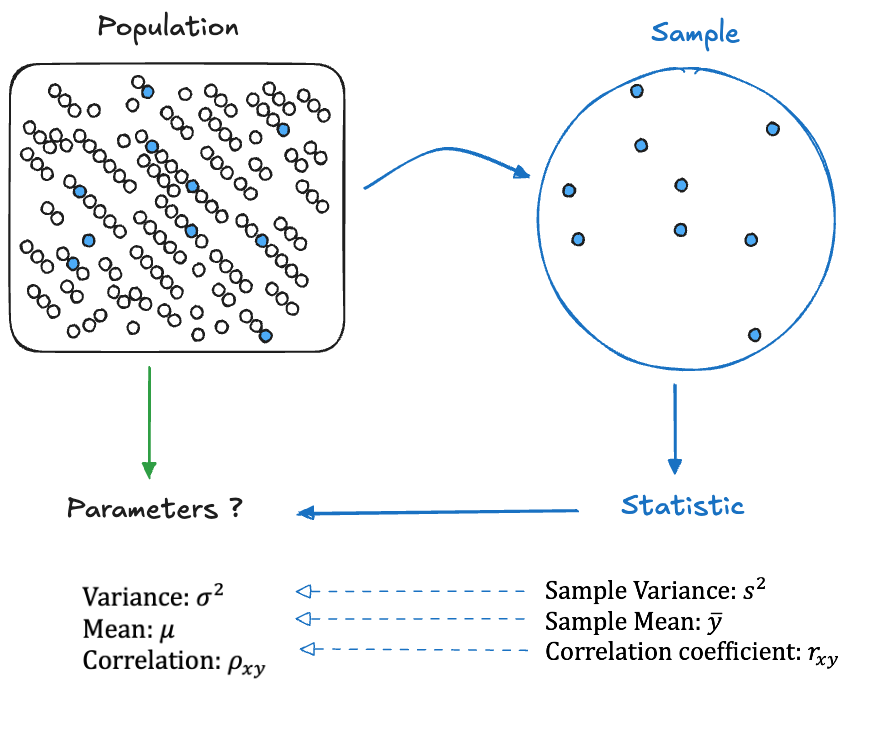
The statistics are random variables because the attribute sampled from the population is not constant, it has variability. Depending on which elements of the population make it into the sample, the values of the statistics will differ. The only ways around the variability in statistics would be to either
- observe (measure) all elements of the population, a procedure known as a census
- observe an attribute that does not vary in the population (\(\text{Var}[Y] = 0\)).
In the first case there is no variability in the statistics because every repetition of the census yields the exact same data. In the second case there is no variability in the statistics because there is no variability in the values we observe. In situation 2 we might as well just sample a single observation and we know everything there is to know about the attribute in question.
Random Variables & Realizations
When discussing statistics, the quantities computed from data, we must make a distinction between random quantities and their realizations. For example, suppose you draw \(n\) observations from a Gaussian distribution with mean \(\mu\) and variance \(\sigma^2\). This is the same as saying that there is a population where attribute \(Y\) follows a \(G(\mu, \sigma^2)\) distribution and we are pulling a random sample of \(n\) elements of the population.
What is the difference between the following quantities \[ \begin{align*} \overline{Y} &= \frac{1}{n} \sum_{i=1}^n Y_i \\ \overline{y} &= \frac{1}{n} \sum_{i=1}^n y_i \end{align*} \]
The distributional properties of \(Y\) in the population can be expressed as \(Y \sim G(\mu,\sigma^2)\). \(Y_1\) is the first random variable in our sample. \(y_1\) is the value
observed on the first draw, for example, \(y_1 = 5.6\).
When we refer to the random variables, we use upper-case notation, when we refer to their realized (observed) values in a particular set of data we use lower-case notation. Both \(\overline{Y}\) and \(\overline{y}\) refer to the sample mean. \(\overline{Y}\) is a random variable, \(\overline{y}\) is the actual value of the sample mean in our data, it is a constant. \(\overline{Y}\) has an expected value (the mean of the sample mean) and a variance that are functions of the mean and variance of the population from which the sample is drawn,
\[\begin{align*} \text{E}\left[ \overline{Y}\right] &= \mu \\ \text{Var} \left[\overline{Y}\right] &= \frac{\sigma^2}{n} \end{align*}\]
The variance of \(\overline{y}\) is zero, and its expected value is equal to the value we obtained for \(\overline{y}\), because it is a constant:
\[\begin{align*} \text{E}\left[ \overline{y}\right] &= \overline{y} \\ \text{Var} \left[\overline{y}\right] &= 0 \end{align*}\]
It should always be clear from context whether we are talking about the random properties of a statistic or its realized value. Unfortunately, notation is not always clear. In statistical models, for example, it is common to use Greek letters for parameters. These are unknown constants. Based on data we find estimators for the parameters. For example, in the simple linear regression model \[ Y_i = \beta_0 + \beta_1 x_i + \epsilon_i \] \(\beta_0\) and \(\beta_1\) are the intercept and slope parameters of the model. The ordinary least squares estimator of \(\beta_1\) is \[ \widehat{\beta}_1 = \frac{S_{xy}}{S_{xx}} = \frac{\sum_{i=1}^n (x_i - \overline{x})(Y_i - \overline{Y})}{\sum_{i=1}^n(x_i - \overline{x})^2} \tag{60.1}\]
The input variable is considered fixed in regression models, not a random variable. That is why we use lower-case notation for \(x_i\) and \(\overline{x}\) in Equation 60.1. With respect to the target variable we have two choices. Equation 60.1 uses upper-case notation, referring to the random variables. \(\widehat{\beta}_1\) in Equation 60.1 is a random variable and we can study the distributional properties of \(\widehat{\beta}_1\).
The expression for \(\widehat{\beta}_1\) in Equation 60.2 uses lower-case notation for \(y_i\) and \(\overline{y}\), it is referring to the constants computed from a particular sample.
\[ \widehat{\beta}_1 = \frac{S_{xy}}{S_{xx}} = \frac{\sum_{i=1}^n (x_i - \overline{x})(y_i - \overline{y})}{\sum_{i=1}^n(x_i - \overline{x})^2} \tag{60.2}\]
The quantity \(\widehat{\beta}_1\) in Equation 60.2 is the realized value of the regression slope, for example, 12.456. Unfortunately, the notation \(\widehat{\beta}_1\) does not tell us whether we are referring to the estimator of the slope—a random variable—or the estimate of the slope—a constant.
Two primary lines of inquiry in statistics are the description of data—through quantitative and visual summaries—and the drawing of conclusions from data. These lines of inquiry are called descriptive and inferential statistics. Descriptive statistics—the discipline—describes the features of a population (a distribution) based on the data in a sample. Inferential statistics—the discipline—draws conclusions about one or more populations.
Both lines of inquiry rely on statistics, quantities computed from data. The distinction lies in how the statistics are used. Descriptive statistics uses the sample mean to estimate the central tendency—the typical value—of a population. Inferential statistics uses the sample means in two groups to conclude whether the means of the populations are different.
60.2 Descriptive Statistics
Descriptive statistics capture the feature of a distribution (a population) in numerical or graphical summaries. The most important features of a distribution are its central tendency (location) and its variability (dispersion). The central tendency captures where the typical values are located, the dispersion expresses how much the distribution spreads around the typical values.
Numerical Summaries
Table 60.1 shows important location statistics and Table 60.2 important dispersion statistics.
| Sample Statistic | Symbol | Computation | Notes |
|---|---|---|---|
| Min | \(Y_{(1)}\) | The smallest non-missing value | |
| Max | \(Y_{(n)}\) | The largest value | |
| Mean | \(\overline{Y}\) | \(\frac{1}{n}\sum_{i=1}^n Y_i\) | Most important location measure, but can be affected by outliers |
| Trimmed Mean | \(\tilde{Y}_p\) | Remove \(p\)% of the observations in each tail of the sample and compute the sample mean of the remainder. Robust against outliers. | |
| Median | Med | \(\left \{ \begin{array}{cc} Y_{\left(\frac{n+1}{2}\right)} & n \text{ is even} \\ \frac{1}{2} \left( Y_{\left(\frac{n}{2} \right)} + Y_{\left(\frac{n}{2}+1\right)} \right) & n\text{ is odd} \end{array}\right .\) | Half of the observations are smaller than the median; robust against outliers |
| Mode | Mode | The most frequent value; not useful when real numbers are unique. Appropriate measure for nominal data. | |
| 1st Quartile | \(Q_1\) | \(Y_{\left(\frac{1}{4}(n+1) \right)}\) | 25% of the observations are smaller than \(Q_1\) |
| 2nd Quartile | \(Q_2\) = Med | See Median | 50% of the observations are smaller than \(Q_2\). This is the median |
| 3rd Quartile | \(Q_3\) | \(Y_{\left(\frac{3}{4}(n+1) \right)}\) | 75% of the observations are smaller than \(Q_3\) |
| X% Percentile | \(Y_{\left(\frac{X}{100}(n+1) \right)}\) | For example, 5% of the observations are larger than \(P_{95}\), the 95% percentile |
The most important location measures are the sample mean \(\overline{Y}\) and the median. The sample mean is the arithmetic average of the sample values. Because the sample mean can be affected by outliers—large values are pulling the sample mean up—the median is preferred in the presence of extreme observations. For example, when reporting central tendency of annual income, the median income is chosen over the arithmetic average so that extreme incomes like those of Elon Musk, Jeff Bezos, and Mark Zuckerberg do not distort the notion of the typical value.
| Sample Statistic | Symbol | Computation | Notes |
|---|---|---|---|
| Range | \(R\) | \(Y_{(n)} - Y_{(1)}\) | \(n\)th order statistic (largest) minus first (smallest) order statistic |
| Inter-quartile Range | IQR | \(Q_3 - Q_1\) | Used in constructing box plots; covers the central 50% of the data |
| Standard Deviation | \(S\) | \(\sqrt{\frac{1}{n-1}\sum_{i=1}^n\left( Y_i - \overline{Y}\right)^2}\) | Most important dispersion measure; in the same units as the sample mean (the units of \(Y\)) |
| Variance | \(S^2\) | \(\frac{1}{n-1}\sum_{i=1}^n \left( Y_i - \overline{Y} \right)^2\) | Important statistical measure of dispersion; in squared units of \(Y\) |
| Skewness | \(g_1\) | \(\frac{\frac{1}{n}\sum_{i=1}^n(Y_i - \overline{Y})^3}{S^3}\) | Measures the symmetry of a distribution |
| Kurtosis | \(k\) | \(\frac{\frac{1}{n}\sum_{i=1}^n(Y_i - \overline{Y})^4}{S^4}\) | Measures the peakedness of a distribution |
Graphical Summaries
We view a population as a distribution of values. Data visualizations thus lend themselves to the description of populations. The more important visual descriptive summaries are the frequency distribution (histogram) and the boxplot.
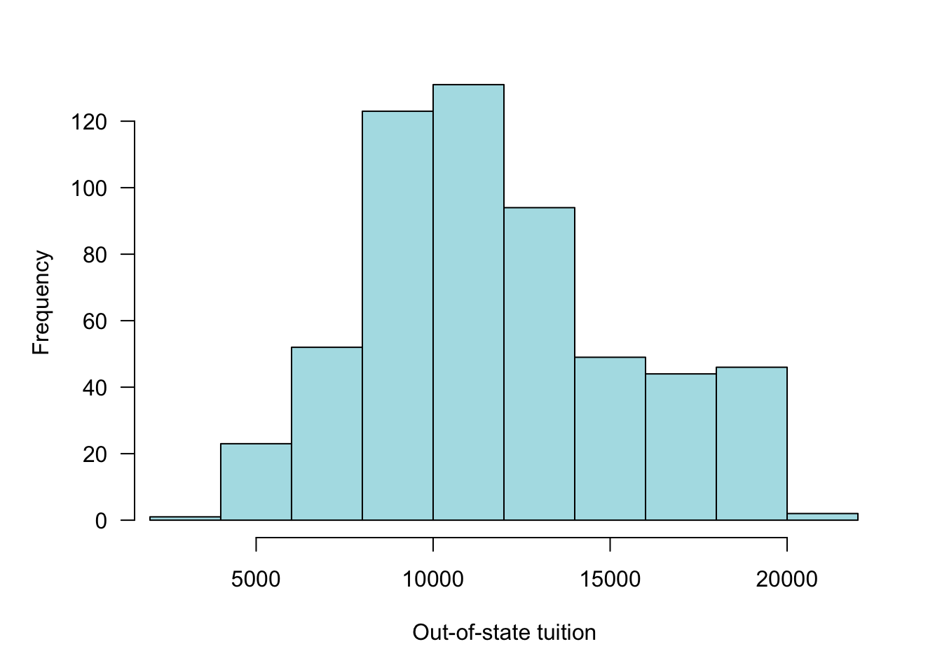
Histogram (Frequency Distribution)
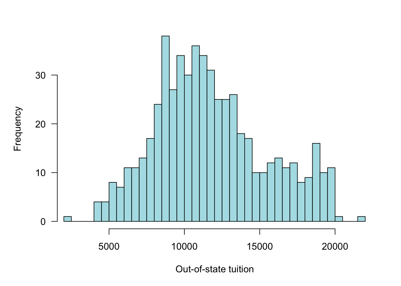
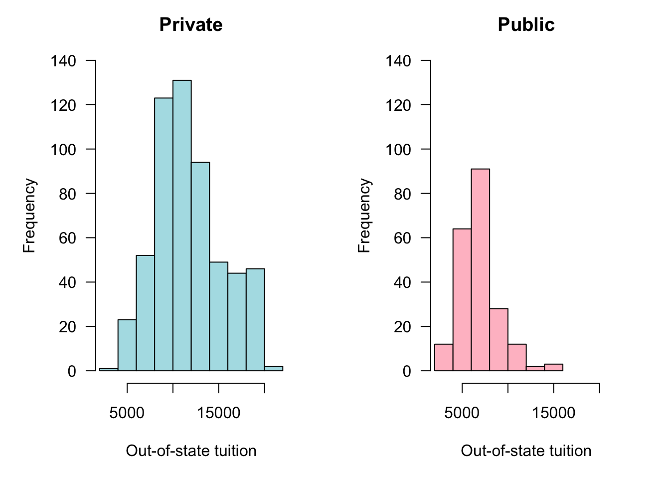
The frequency distribution is constructed by binning the observed values into segments of equal width. Figure 60.2 shows the (absolute) frequency distribution of out-of-state tuition for private universities in 1995. Figure 60.3 displays the same data with a large number of frequency bins (30). Between 5 and 30 bins is typical for histograms. The number of bins should not be too small to obscure features of the distribution and it should not be too large to create artifacts in regions of low data density.
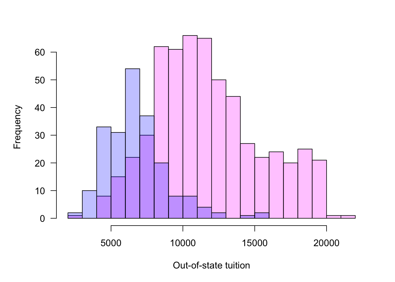
To compare frequency distributions between groups, histograms can be plotted side by side or overlaid. When the histograms overlap, a side-by-side display is preferred because bars from different groups can obscure it each other. Adding transparency to the bars helps but can still create confusing displays (Figure 60.4).
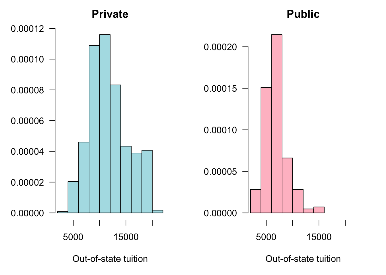
In the side-by-side display attention needs to be paid to the scale of the horizontal and vertical axes. Figure 60.5 forces the axes to be the same in both histograms to facilitate a direct comparison. Alternatively to forcing the vertical axes to the same frequency range you can express the frequencies in relative terms (Figure 60.6).
Boxplot
The boxplot, also called the box-and-whisker plot, is a simple visualization of a distribution that combines information about location, dispersion, and extreme values. The standard boxplot (Figure 60.7) comprises
- a box that covers the inter-quartile range from \(Q_1\) to \(Q_3\).
- a line through the box at the location of the median (\(Q_2\)).
- Whiskers that extend from the edge of the box to the largest and smallest observations within \(1.5\times \text{IQR}\).
- Outliers that fall outside the whiskers.
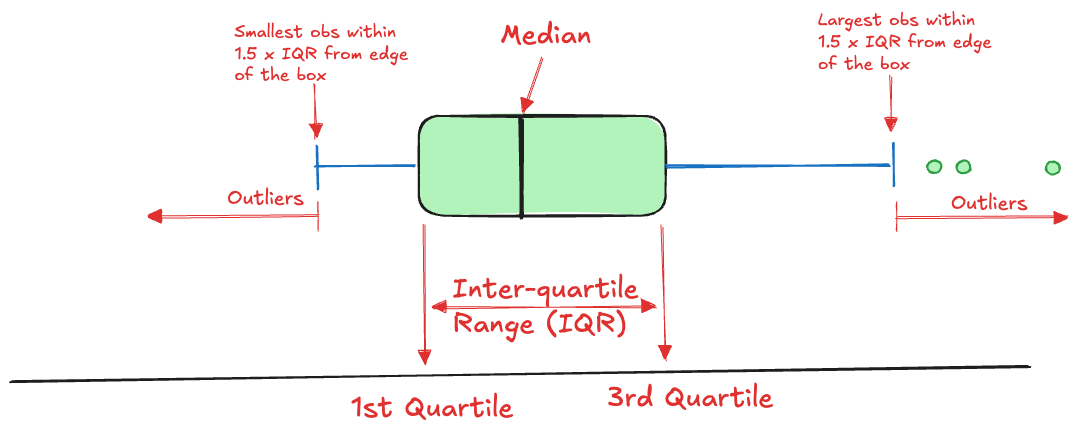
The idea of the boxplot is that the box covers the central 50% of the observation, the whiskers extend to the vast majority of the data. Data points that fall outside the whiskers are declared outliers.
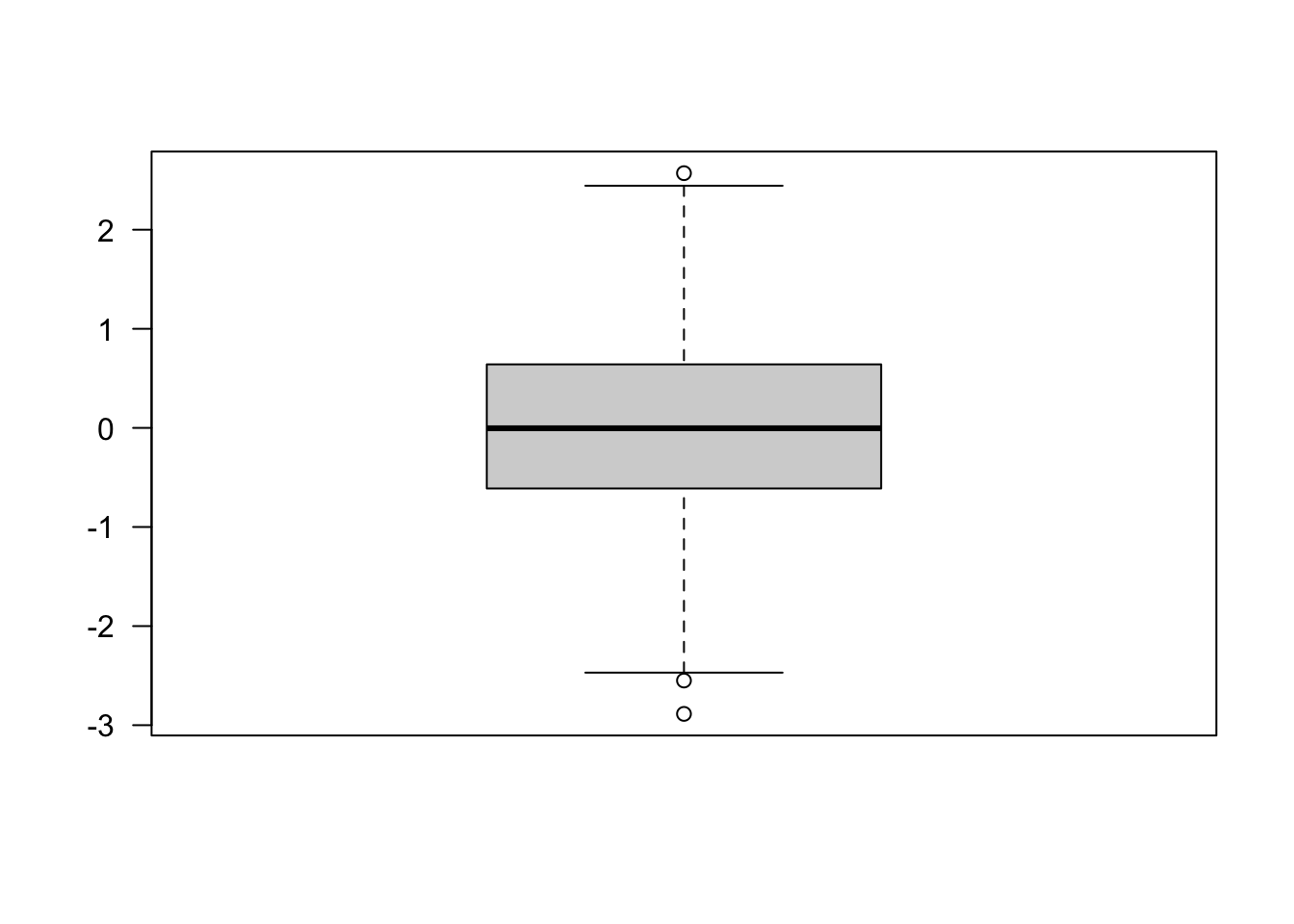
Note, however, that outlying observations in a boxplot does not necessarily indicate observations that are inconsistent with the data. A boxplot for a sample from a normal distribution will likely show some outliers by this definition (Figure 60.8). The probability to observe values outside of the whiskers for a \(G(\mu,\sigma^2)\) distribution is 0.00697. In a sample of \(n=1000\) you should expect to see 7 observations beyond the whiskers.
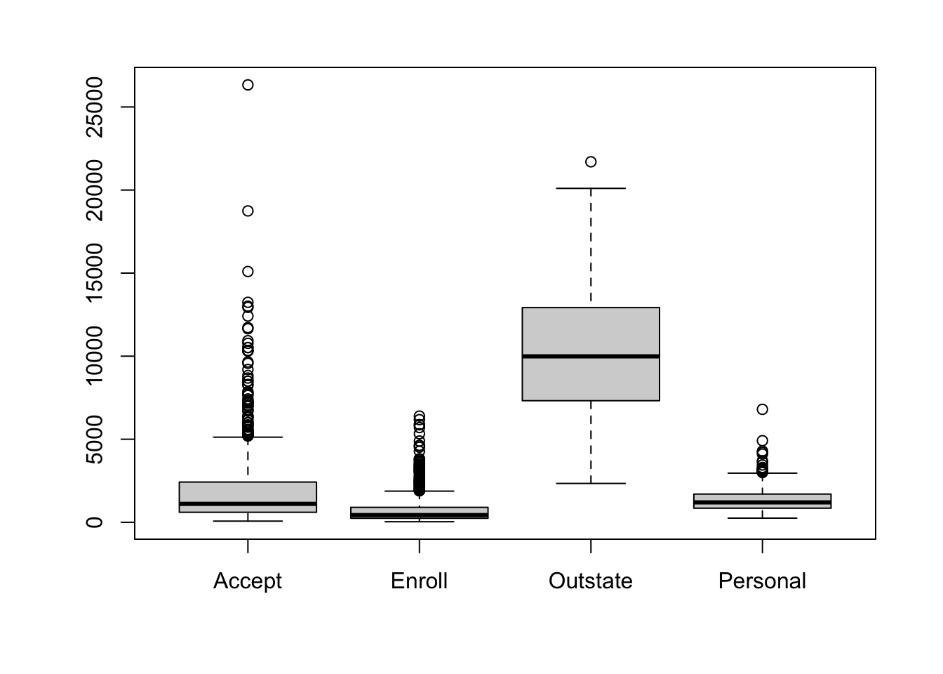
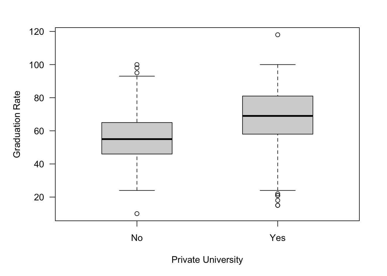
Boxplots are great visual devices to compare the distribution for different attributes (Figure 60.9) or to compare the same attribute across different groups (Figure 60.10).
60.3 Sampling Distributions
Sampling distributions are probability distributions of statistics computed from random samples.
Chapter 59 discussed probability distributions in general. If one draws a random sample from, say, a \(G(\mu,\sigma^2)\) distribution, what are the distributional properties of statistics like \(\overline{Y}\), \(S^2\), and so on?
We know that \(\overline{Y}\) in a random sample from a distribution with mean \(\mu\) and variance \(\sigma^2\) has mean \(\text{E}[\overline{Y}] = \mu\) and variance \(\text{Var}[\overline{Y}] = \sigma^2/n\). This can be verified based on properties of expected values in iid samples. We do not need to mess with any density or mass functions.
\[ \begin{align*} \text{E}\left[\overline{Y}\right] &= \frac{1}{n}\text{E}\left[\sum_{i=1}^n Y_i\right] = \frac{1}{n} \sum_{i=1}^n \text{E}\left[Y_i\right] \\ &= \frac{1}{n} \sum_{i=1}^n \mu = \frac{n\mu}{n} = \mu \end{align*} \tag{60.3}\]
\[ \begin{align*} \text{Var}\left[\overline{Y} \right] &= \text{Var}\left[ \frac{1}{n}\sum_{i=1}^n Y_i \right]\\ &= \frac{1}{n^2} \text{Var} \left[ \sum_{i=1}^n Y_i \right]\\ &= \frac{1}{n^2} \sum_{i=1}^n \text{Var}\left[ Y_i \right]\\ &= \frac{1}{n^2} \sum_{i=1}^n \sigma^2 = \frac{n\sigma^2}{n^2} = \frac{\sigma^2}{n} \end{align*} \tag{60.4}\]
Equation 60.3 and Equation 60.4 apply to any population, as long as we draw a random sample. What else can we say about the distribution of \(\overline{Y}\)?
Central Limit Theorem
By the central limit theorem, introduced at the end of the previous chapter, we can say that the distribution of \[ \frac{\overline{Y} - \mu}{\sigma/\sqrt{n}} \] converges to a \(G(0,1)\) distribution as \(n\) grows to infinity. Another way of saying this is that the distribution of \(\overline{Y}\) converges to a \(G(\mu,\sigma^2/n)\) distribution.
This is a pretty amazing result. Regardless of the shape of the population you are sampling from, whether the attribute is continuous or discrete, if you draw a large enough sample, the sample mean will behave like a Gaussian random variable where the mean is the same as that of the population and the variance is \(n\)-times smaller than the population variance.
Example: Distribution of Sample Mean of Bernoullis
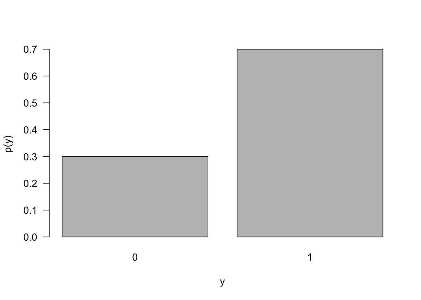
The distribution furthest from a Gaussian distribution in some sense is the Bernoulli(\(\pi\)) distribution. It is a discrete distribution with only two outcomes. Only for \(\pi=0.5\) is the Bernoulli distribution symmetric. Figure 60.11 shows the mass function of a Bernoulli distribution with \(\pi=0.7\). How do you go from that to a continuous, symmetric Gaussian distribution?
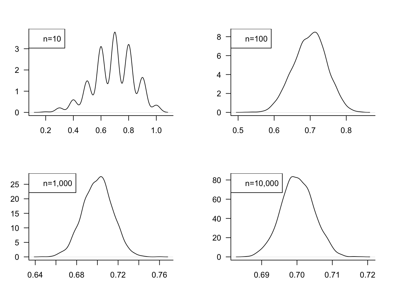
Let’s study the distribution of the sample mean if we draw random samples of sizes \(n_1 = 10\), \(n_2=100\), \(n_3 = 1000\), and \(n_4=10000\) from a Bernoulli(0.7). In order to get a good estimate of the sampling distribution of \(\overline{Y}\) the process needs to be repeated a sufficient number of times. We choose \(m=2500\) repetitions of the experiment to build up the distribution of \(\overline{Y}\).
Figure 60.12 shows the sampling distributions of \(\overline{Y}\) for the four sample sizes. For \(n=10\), for example, a random sample of size 10 was drawn from a Bernoulli(0.7) and its sample mean was calculated. This was repeated another 2,499 times and the figure displays the estimated probability density of the 2,500 \(\overline{y}\) values. A similar procedure for the other sample sizes leads to the respective density estimates.
With \(n=10\), the distribution is far from Gaussian. The sample mean can take on only 10 possible values, \(0, 0.1, 0.2, \cdots, 1.0\). As \(n\) increases, the number of possible values of \(\overline{Y}\) increases, the distribution becomes more continuous. It also becomes more symmetric and approaches the Gaussian distribution. For a sample of size \(n=1000\), the sample mean is very nearly Gaussian distributed and increasing the sample size to \(n=10,000\) does not appear to improve the quality of the Gaussian approximation much. However, it does increase the precision of \(\overline{Y}\) as an estimator; the variance of the sampling distribution for \(n=10,000\) is less than the variance of the sampling distribution for \(n=1,000\). We can calculate the variance of the sample mean in this case based on Equation 60.4:
\[ \text{Var}\left[\overline{Y}\right] = \frac{0.7 \times 0.3}{10000} = 0.000021 \]
Sampling from a Gaussian
The central limit theorem specifies how the distribution of \(\overline{Y}\) evolves as more and more samples are drawn. If the distribution we sample from is itself Gaussian, we do not need a large-sample approximation to describe the distribution of \(\overline{Y}\).
In a random sample of size \(n\) from a \(G(\mu,\sigma^2)\) distribution, the distribution of \(\overline{Y}\) follows a \(G(\mu,\sigma^2/n)\) distribution. In other words, the distribution of \(\overline{Y}\) is known to be exactly Gaussian, regardless of the size of the sample. As long as we draw a random sample—that is, the random variables are iid.
In parallel to how the central limit theorem was stated above, we can say that if \(Y_1, \cdots, Y_n\) are iid \(G(\mu,\sigma^2)\), then \[ \frac{\overline{Y}-\mu}{\sigma/\sqrt{n}} \sim G(0,1) \tag{60.5}\]
The Gaussian distribution is just one of several important distributions we encounter when working with statistics computed from Gaussian samples, The \(t\), \(\chi^{2}\), and \(F\) distributions are other important sampling distributions. These distributions play an important role in inferential statistics, for example in computing confidence intervals or testing hypotheses about parameters. Names such as \(t\)-test, \(F\)-test, or chi-square test stem from the distribution of statistics used to carry out the procedure.
Chi-Square Distribution, \(\chi^2_\nu\)
Let \(Z_{1},\cdots,Z_{k}\) denote independent standard Gaussian random variables \(G(0,1)\). Then
\[ X = Z_{1}^{2} + Z_{2}^{2} + \cdots + Z_{k}^{2} \]
has p.d.f.
\[ f(x) = \frac{1}{2^{\frac{k}{2}}\Gamma\left( \frac{k}{2} \right)}x^{\frac{k}{2}}e^{- x/2},\ \ \ \ \ x \geq 0 \]
This is known as the Chi-square distribution with \(k\) degrees of freedom, abbreviated \(\chi_{k}^{2}\). The mean and variance of a \(\chi_{k}^{2}\) random variable are \(\text{E}\lbrack X\rbrack = k\) and \(\text{Var}\lbrack X\rbrack = 2k\).
The degrees of freedom can be thought of as the number of independent pieces of information that contribute to the \(\chi^{2}\) variable. Here, that is the number of independent \(G(0,1)\) variables. Since the \(\chi^{2}\) variable is the sum of their squared values, the density shifts more to the right as the degrees of freedom increase (Figure 60.13).
\(\chi^{2}\) distributions are important to capture the sample distributions of dispersion statistics. If \(Y_{1},\cdots,Y_{n}\) are a random sample from a \(G\left( \mu,\sigma^{2} \right)\) distribution, and the sample variance is
\[ S^2 = \frac{1}{n-1}\sum_{i=1}^n\left( Y_i - \overline{Y} \right)^2 \] then the random variable \[ \frac{(n-1)S^2}{\sigma^2} \] follows a \(\chi_{n-1}^2\) distribution. It follows that \(S^2\) is an unbiased estimator of \(\sigma^2\):
\[ \text{E}\left\lbrack \frac{(n-1)S^2}{\sigma^2} \right\rbrack = n - 1 \]
\[ \text{E}\left\lbrack S^{2} \right\rbrack = \sigma^2 \]
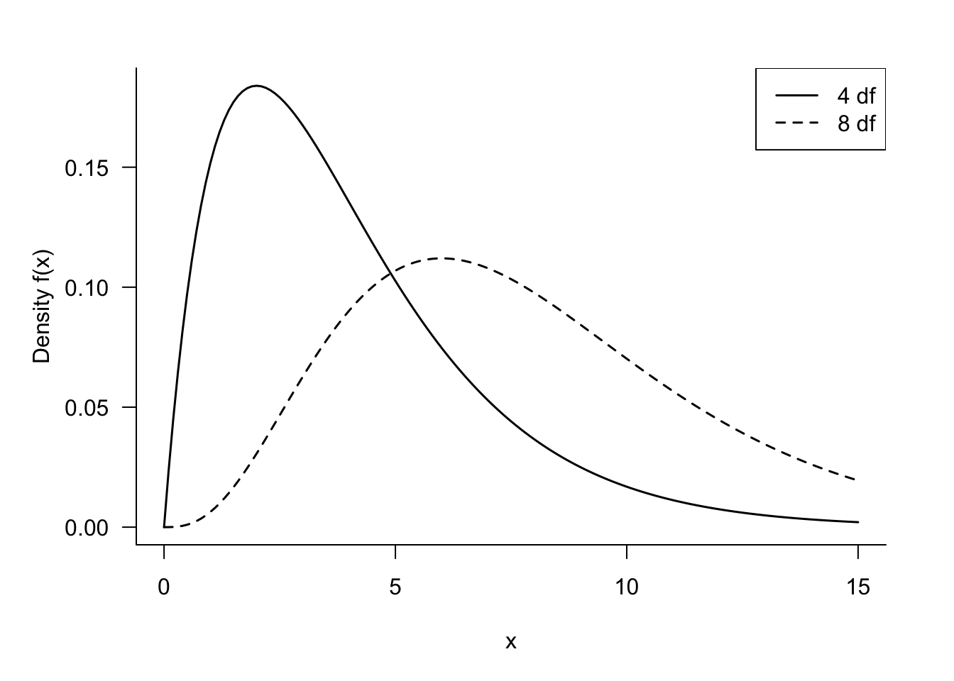
Students’ t Distribution, \(t_\nu\)
In the Gaussian case you can also show that \(\overline{Y}\) and \(S^2\) are independent random variables. This is important because of another distributional result: if \(Z \sim G(0,1)\) and \(U \sim \chi_\nu^2\), and \(Z\) and \(U\) are independent, then the ratio
\[ T = \frac{Z}{\sqrt{U/\nu}} \]
has a \(t\) distribution with \(\nu\) degrees of freedom. In honor of Student, the pseudonym used by William Gosset for publishing statistical research while working at Guinness Breweries, the \(t\) distribution is also known as Student’s \(t\) distribution or Student’s distribution for short.
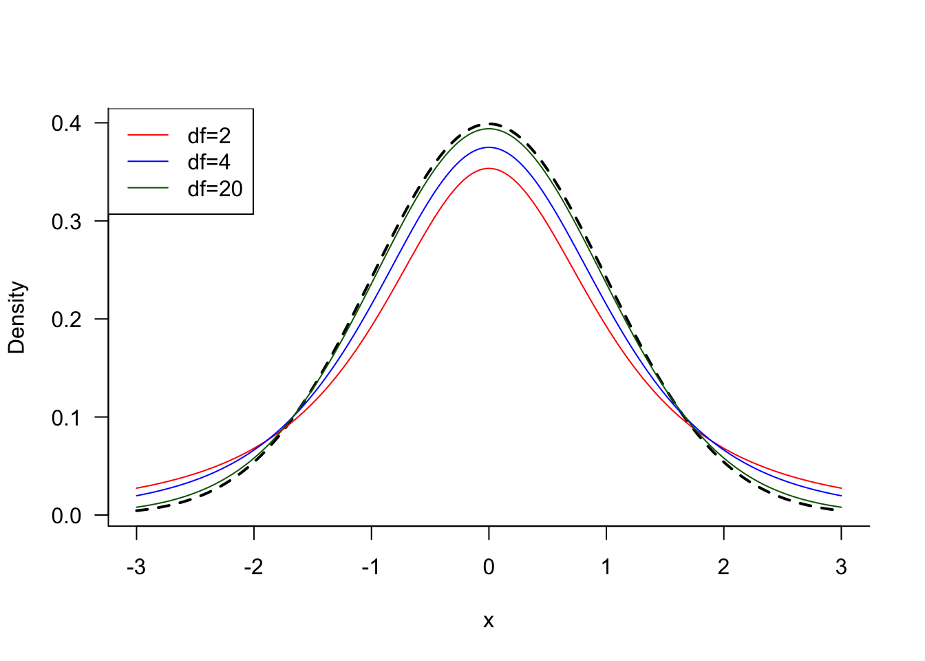
As with the \(\chi_\nu^2\) distributions, the shape of the \(t_\nu\) distribution depends on the degrees of freedom \(\nu\). However, the \(t_\nu\) distributions are symmetric about zero and the degrees of freedom affect how heavy the tails are. As the degrees of freedom grow, the \(t\) density approaches that of the standard Gaussian distribution (Figure 60.14).
We can now combine the results about the sampling distributions of \(\overline{Y}\) and \(S^2\) to derive the distribution of
\[ \frac{\overline{Y} - \mu}{S/\sqrt{n}} \tag{60.6}\]
We know that \(\overline{Y} \sim G\left( \mu,\frac{\sigma^2}{n} \right)\) and that \(\frac{(n-1)S^2}{\sigma^2}\) follows a \(\chi_{n-1}^2\) distribution. Furthermore, \(\overline{Y}\) and \(S^2\) are independent. Taking ratios as required by the definition of a \(t\) random variable yields
\[ \frac{\frac{\overline{Y} - \mu}{\sigma/\sqrt{n}}}{\sqrt{S^2{/\sigma}^2}} = \frac{\overline{Y} - \mu}{S/\sqrt{n}} \sim t_{n - 1} \]
Compare Equation 60.5 to Equation 60.6. The difference is subtle, the dispersion statistic in the denominator. If the population variance \(\sigma^2\) is known, we use Equation 60.5 and the distribution is Gaussian with mean 0 and variance 1. If \(\sigma^2\) is unknown, we replace \(\sigma\) in Equation 60.5 with an estimator based on the sample, the sample standard deviation \(S\). The result is a \(t\) distribution with \(n-1\) degrees of freedom. As \(n\) increases, the \(t\) distribution approaches a \(G(0,1)\) distribution because the estimator \(S\) approaches a constant. For any given value \(n\), the \(t\) distribution will be heavier in the tails than a \(G(0,1)\) distribution because there is more uncertainty in the system when the random variable \(S\) is used as an estimator of the constant \(\sigma\) (Figure 60.14).
F Distribution, \(F_{\nu_1, \nu_2}\)
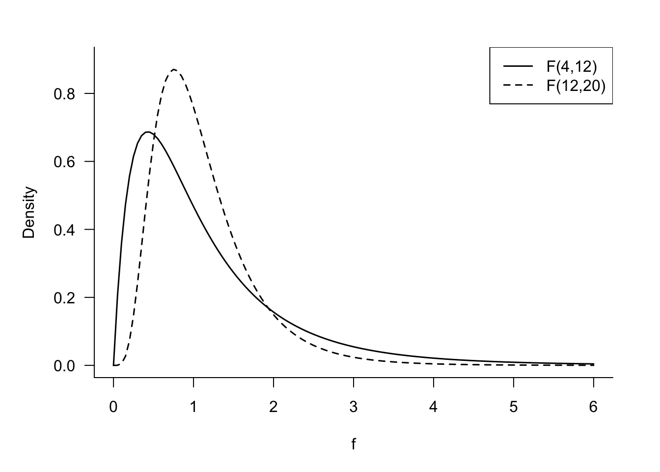
If \(\chi_1^2\) and \(\chi_2^2\) are independent chi-square random variables with \(\nu_1\) and \(\nu_2\) degrees of freedom, respectively, then the ratio
\[ F = \frac{\chi_1^2/v_1}{\chi_2^2/\nu_2} \]
follows an \(F\) distribution with \(\nu_1\) numerator and \(\nu_2\) denominator degrees of freedom (Figure 60.15). We denote this fact as \(F\sim F_{\nu_1,\nu_2}\). The mean and variance of the \(F\) distribution are
\[ \begin{align*} \text{E}\lbrack F\rbrack &= \frac{\nu_2}{\nu_{2} - 2} \\ \text{Var}\lbrack F\rbrack &= \frac{2\nu_2^2 (\nu_1 + \nu_2 + 2)}{\nu_1\left( \nu_2 - 2 \right)^2 (\nu_2 - 4)} \end{align*} \]
The mean exists only if \(\nu_{2} > 2\) and the variance exists only if \(\nu_{2} > 4\).
When sampling from a Gaussian distribution we established that \(\frac{(n-1)S^2}{\sigma^2}\) follows a \(\chi_{n-1}^{2}\) distribution. Suppose we have two samples, one of size \(n_1\) from a \(G(\mu_1,\sigma_1^2)\) distribution and one of size \(n_2\) from a \(G(\mu_2,\sigma_2^2)\) distribution. If the estimators of the sample variances in the two samples are denoted \(S_1^2\) and \(S_2^2\), respectively, then the ratio
\[ \frac{S_1^2/\sigma_1^2}{S_2^2/\sigma_2^2} \]
has an \(F_{n_1-1,n_2-1}\) distribution.
\(F\) distributions play an important role in the analysis of variance, where the numerator and denominator are ratios of mean squares.
Recall that the \(T\) random variable in the Gaussian case can be written as
\[ T = \frac{\frac{\overline{Y} - \mu}{\sigma/\sqrt{n}}}{\sqrt{S^2{/\sigma}^2}} \]
The numerator is a \(G(0,1)\) variable, so squaring it yields a \(\chi_1^2\) variable. The square of the denominator is a scaled \(\chi_{n-1}^2\) variable, \(S^2/\sigma^2\). Also, because \(\overline{Y}\) and \(S^2\) are independent, the squares of the numerator and denominator are independent. It thus follows that
\[ T^2 = \frac{\left( \overline{Y} - \mu \right)^2}{S^2/n}\]
follows an \(F_{1,n - 1}\) distribution.
This fact is used in software packages that report the result of an \(F\)-test instead of the result of a two-sided \(t\)-test. The two are equivalent and the \(p\)-values are the same.
60.4 Inferential Statistics
The process of statistical inference is to draw conclusions about the world based on data. The world is described in terms of populations and the probability distributions of attributes in the population. The data consists of observations drawn from those populations, random variables that follow the distribution laws that govern the populations. The goal is to infer properties of the populations based on the information captured in the data.
Some of the statistics computed in inference procedures are the same used to describe populations (distributions). For example, the sample mean describes the central tendency of a distribution, it is also used to compute confidence intervals for the mean in the population. Statistical inference adds a further dimension to describing things; it investigates the properties of the statistics such as bias and variance.
Point Estimation
A point estimate is a single number to estimate a parameter. The corresponding statistic is the point estimator. \(\overline{y} = 10.4\) in a random sample is the point estimate for the mean \(\mu\). \(\overline{Y} = \frac{1}{n}\sum_{i=1}^n Y_i\) is the point estimator; a rule that tells how to calculate the estimate.
Important properties of a point estimator are the bias and variance. The bias is a measure of its accuracy. An unbiased estimator is an accurate estimator. The variance is a measure of the uncertainty associated with the estimator; it is the reciprocal of the estimator’s precision. A highly variable estimator is not precise—and vice versa.
Bias and variance are long-run properties of the estimator, they are expected values.
Definition: Bias, Variance, and Mean Squared Error
The bias of an estimator is the expected value of the difference between the estimator and the parameter it is estimating. If \(\theta\) is the parameter of interest and \(h(\textbf{Y})\) is an estimator—a function of \(\textbf{Y}=[Y_1,\cdots,Y_n]^\prime\)—then \[ \text{Bias}\left[h(\textbf{Y});\theta\right] = \text{E}\left[h(\textbf{Y})-\theta\right] = \text{E}\left[h(\textbf{Y})\right]-\theta \] The variance of an estimator is the usual expected squared difference between the estimator and its mean: \[ \text{Var}[h(\textbf{Y})] = \text{E}\left[\left(h(\textbf{Y})-\text{E}[h(\textbf{Y})]\right)^2\right] \] The mean squared error of estimator \(h(\textbf{Y})\) for the parameter \(\theta\) is \[ \text{MSE}\left[h(\textbf{Y});\theta\right] = \text{E}\left[\left(h(\textbf{Y})-\theta\right)^2 \right] = \text{Var}[h(\textbf{Y})] + \text{Bias}\left[h(\textbf{Y});\theta\right]^2 \tag{60.7}\]
An estimator with \(\text{Bias}[h(\textbf{Y});\theta] = 0\) is said to be unbiased for \(\theta\). An unbiased estimator that has the smallest variance among all unbiased estimators is said to be a uniform minimum variance unbiased estimator (UMVUE).
Estimators with small bias and a sharply reduced variance—compared to the best unbiased estimator—can have a smaller mean squared error and can thus be preferred over an unbiased estimator.
Example: Estimating the Parameter of an Exponential Distribution
Suppose that \(Y\) has an exponential distribution with density \[ f(y) = \frac{1}{\theta} \, e^{-y/\theta}\qquad \text{for } y > 0 \] This is a re-parameterization of the density in Section 59.5.2 where \(\theta = 1/\lambda\). The mean and variance of \(Y\) are \(\text{E}[Y] = \theta\) and \(\text{Var}[Y] = \theta^2\). You draw a random sample of size \(n=3\). Consider the following estimators:
- \(\widehat{\theta}_1 = Y_1\)
- \(\widehat{\theta}_2 = \frac{Y1+Y2}{2}\)
- \(\widehat{\theta}_3 = \frac{Y1+2Y2}{3}\)
- \(\widehat{\theta}_4 = \overline{Y}\)
- \(\widehat{\theta}_5 = \min\{Y1,Y2,Y3\}\)
Which of these estimators are unbiased, which one has the smallest variance and mean squared error?
It is easy to establish that \(\widehat{\theta}_1\) through \(\widehat{\theta}_4\) are unbiased: \[ \begin{align*} \text{E}\left[\widehat{\theta}_1\right] &= \text{E}[Y_1] = \theta \\ \text{E}\left[\widehat{\theta}_2\right] &= \frac{1}{2}(\text{E}[Y_1] + \text{E}[Y_2])= \frac{2\theta}{2} = \theta \\ \text{E}\left[\widehat{\theta}_3\right] &= \frac{1}{3}(\text{E}[Y_1] + 2\text{E}[Y_2])= \frac{3\theta}{3} = \theta \\ \text{E}\left[\widehat{\theta}_4\right] &= \frac{1}{3}(\text{E}[Y_1] + \text{E}[Y_2] + \text{E}[Y_3])= \frac{3\theta}{3} = \theta \\ \end{align*} \]
The variances of these estimators are \[ \begin{align*} \text{Var}\left[\widehat{\theta}_1\right] &= \text{Var}[Y_1] = \theta^2 \\ \text{Var}\left[\widehat{\theta}_2\right] &= \frac{1}{4}(\text{Var}[Y_1] + \text{Var}[Y_2])= \frac{2}{4}\theta^2 = \frac{1}{2}\theta^2 \\ \text{Var}\left[\widehat{\theta}_3\right] &= \frac{1}{9}(\text{Var}[Y_1] + 4\text{Var}[Y_2])= \frac{5}{9}\theta^2 \\ \text{Var}\left[\widehat{\theta}_4\right] &= \frac{1}{3}\theta^2 \end{align*} \] The sample mean \(\widehat{\theta}_4\) is the most precise (smallest variance) estimator among the first four.
To find the properties of \(\widehat{\theta}_5 = \min\{Y_1,Y_2,Y_3\}\) a bit more work is required. This is called the first order statistic, the smallest value in the sample. It is denoted as \(Y_{(1)}\). The largest value, the \(n\)th order statistic, is denoted \(Y_{(n)}\). You can show that the first order statistic in a random sample of size \(n\) has density function \[ f_{(1)}(y) = n\left(1-F(y)\right)^{n-1}f(y) \] where \(f(y)\) and \(F(y)\) are the density and cumulative distribution function of \(Y\). For the case of a sample of size \(n\) from an exponential distribution we get \[ f_{(1)}(y) = n\left(1-F(y)\right)^{n-1}\,\frac{1}{\theta}e^{-y/\theta} \] Plugging in \(F(y) = 1 - e^{-y/\theta}\) we get \[ \begin{align*} f_{(1)}(y) &= n\left(e^{-y/\theta}\right)^{n-1}\,\frac{1}{\theta}e^{-y/\theta} \\ &= \frac{n}{\theta}e^{yn/\theta} \end{align*} \] The first order statistic from an exponential distribution with parameter \(\theta\) has an exponential distribution with parameter \(\theta/n\).
We can now evaluate the mean and variance of \(\widehat{\theta}_5\):
\[ \begin{align*} \text{E}\left[\widehat{\theta}_5\right] &= \frac{\theta}{3} \\ \text{Var}\left[\widehat{\theta}_5\right] &= \frac{\theta^2}{9} \end{align*} \] The bias of \(\widehat{\theta}_5\) for \(\theta\) is \[ \text{Bias}\left[\widehat{\theta}_5; \theta\right] = \frac{\theta}{3} - \theta = -\frac{2}{3}\theta \] and the mean squared error is \[ \begin{align*} \text{MSE}\left[\widehat{\theta}_5; \theta\right] &= \text{Var}\left[\widehat{\theta}_5\right] + \text{Bias}\left[\widehat{\theta}_5; \theta\right]^2 \\ &= \frac{1}{9}\theta^2 + \frac{4}{9}\theta^2 = \frac{5}{9}\theta^2 \end{align*} \]
In this case the biased estimator \(\widehat{\theta}_5\) has the same mean squared error as the unbiased estimator \(\widehat{\theta}_3\) but has a larger mean squared error as the sample mean \(\widehat{\theta}_4\).
Interval Estimation
A confidence interval (CI) combines information on a point estimator with information about its precision to yield a range of values associated with a certain probability. For example, a 95% confidence interval for the mean of a population or a 99% confidence interval for the difference between two population means, comparing a placebo and a medical treatment.
The probability associated with the confidence interval is called the confidence level. The complement of the confidence level is frequently denoted \(\alpha\), a nod to the relationship between confidence intervals and significance levels in hypothesis testing. The confidence level is then expressed as \((1-\alpha)\times 100\%\).
Interpretation
Before going into the derivation of confidence intervals, a word about the proper interpretation of the interval. First, a confidence interval refers to a parameter or a function of parameters, not a statistic. Second, a confidence interval is associated with a probability (or percentage); typically a large value such as 90%, 95%, or 99%. The result of estimating a two-sided confidence interval is a lower and an upper confidence bound, these are real numbers. For example, a 95% confidence interval for the population mean might be 5.3 to 12.0. A one-sided confidence interval has either an upper bound or a lower bound.
The correct interpretation of a confidence interval is in terms of repetition of the sampling process, as a long-run frequency. If we were to repeat the sampling process over and over, in 95% of those repetitions the 95% confidence interval would include (cover) the true parameter. In 5% of those repetitions the parameter falls outside (is not covered by) the confidence interval.
It is correct to interpret a 95% confidence interval as a random interval that contains the parameter with probability 0.95. The following interpretations of a confidence interval are not correct, although they are common:
The probability that the interval [5.3, 12.0] covers the parameter is 95%.
This interpretation is incorrect because it assigns the probability to the confidence interval calculated from the specific sample.95% of the data fall within the interval.
The confidence interval makes a statement about a parameter. The interpretation is incorrect since it describes the distribution of the data.
Example
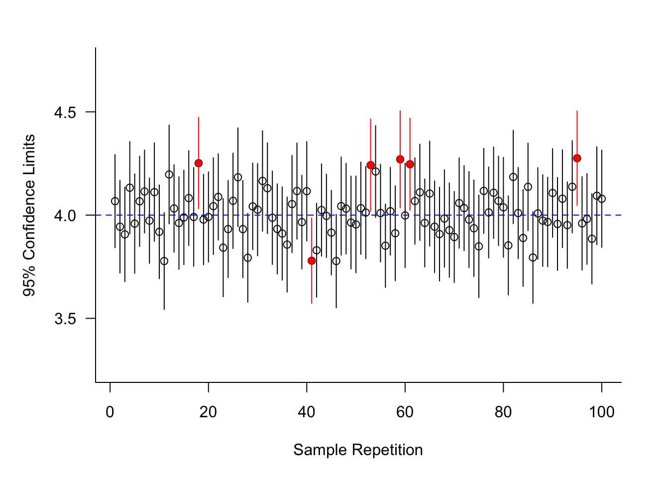
Figure 60.16 displays the result of computing one hundred 95% confidence intervals for the mean of a distribution (population). Since the figure was obtained from a simulation, the value of the unknown mean is known; the mean is \(\mu = 4\).
Under conceptual repetition of the sampling we expect 95% of the confidence intervals to cover the mean. In this particular simulation, computing 100 confidence intervals, 94 of them cover the value \(\mu = 4\) (shown in black), and 6 of the intervals do not cover \(\mu=4\) (shown in red). This is close to the expected, long-run frequency of 95% of intervals covering the parameter.
Constructing confidence intervals
Constructing a confidence interval relies on a statistic and its distribution. The sampling distributions in Section 60.3 play an important role. If we can start from a pivot statistic, constructing confidence interval estimators is pretty easy.
Definition: Pivot Statistic
A pivot statistic for parameter \(\theta\) is a statistic that is a function of \(\theta\) with a known distribution that does not depend on \(\theta\).
Say what? The pivot statistic depends on \(\theta\) but its distribution does not? Exactly, here is an example.
Example: Pivot Statistic for \(\mu\) of a \(G(\mu,\sigma^2)\)
Suppose we want to construct a confidence interval for the mean \(\mu\) of a \(G(\mu,\sigma^2)\) distribution based on the random sample \(Y_1,\cdots,Y_n\). From Section 60.3.4 we know that the statistic \[ T = \frac{\overline{Y}-\mu}{S/\sqrt{n}} \sim t_{n-1} \] has a \(t\) distribution with \(n-1\) degree of freedom.
\(T\) is a proper pivot statistic for calculating a confidence interval for \(\mu\). It depends on \(\mu\) and its distribution does not involve \(\mu\); it does involve \(n\), however, but that is a known quantity (since we know the size of our sample).
The construction of a 95% confidence interval starts with a probability statement. Continuing the example, \[ \Pr\left(t_{0.025,n-1}\leq T\leq t_{0.975,n-1}\right) = 0.95 \]
This simply states that the probability a \(T\) random variable with \(n-1\) degrees of freedom falls between the 2.5% and the 97.5% percentiles is 95%. There are other ways of carving out 95% of the area under the density. The following probability is also true, but it is customary to work with symmetric percentiles, in particular when the pivot distribution is symmetric.
\[ \Pr\left(t_{0.04,n-1}\leq T\leq t_{0.99,n-1}\right) = 0.95 \]
The next step is to substitute the formula for the statistic for \(T\) and to isolate the parameter of interest inside the probability statement.
\[\begin{align*} \Pr\left(t_{0.025,n-1}\leq T\leq t_{0.975,n-1}\right) &= 0.95 \\ \Pr\left(t_{0.025,n-1}\leq \frac{\overline{Y}-\mu}{S/\sqrt{n}}\leq t_{0.975,n-1}\right) &= 0.95\\ \Pr\left(t_{0.025,n-1}\frac{S}{\sqrt{n}}\leq \overline{Y}-\mu\leq t_{0.975,n-1}\frac{S}{\sqrt{n}}\right) &= 0.95\\ \Pr\left(\overline{Y}-t_{0.025,n-1}\frac{S}{\sqrt{n}}\leq \mu\leq \overline{Y}+t_{0.975,n-1}\frac{S}{\sqrt{n}}\right) &= 0.95\\ \end{align*}\]
Now we can peel off the term to the left and the term to the right of the inequalities as the confidence bounds. The 95% confidence interval for the mean of a \(G(\mu,\sigma^2)\) distribution, based on a random sample \(Y_1,\cdots,Y_n\), is \[ \overline{Y} \pm t_{0.975,n-1}\times\frac{S}{\sqrt{n}} \] More generally, the \((1-\alpha)\times 100\)% confidence interval is \[ \overline{Y} \pm t_{\alpha/2,n-1}\times\frac{S}{\sqrt{n}} \]
Confidence intervals based on the CLT
The asymptotic distribution of a statistic can be used to construct confidence intervals when the sample size is sufficiently large. The Central Limit Theorem (CLT) provides the distribution of the pivot statistic.
Suppose \(Y_1,\cdots, Y_n\) is a sample from a Bernoulli(\(\pi\)) distribution and \(n\) is large enough to invoke the CLT. The distribution of the sample mean \(\overline{Y} = 1/n \sum_{i=1}^n Y_i\) converges to a Gaussian distribution with mean \(\pi\) and variance \(\pi(1-\pi)/n\). The sample mean is an unbiased estimate of the event probability \(\pi\).
If \(z_\alpha\) denotes the \(\alpha\) quantile of the \(G(0,1)\) distribution we can state that asymptotically (as \(n\rightarrow\infty\)) \[ \Pr\left(z_{\alpha/2} \leq \frac{\overline{Y}-\pi}{\sqrt{\pi(1-\pi)/n}} \leq z_{1-\alpha/2}\right) \approx 1-\alpha \]
The problem with this interval is that \(\pi\) appears in the numerator and the denominator of the pivot statistic. Proceeding as in the case of the \(t\)-interval leads to \[ \Pr\left(\overline{Y} - \frac{z_{\alpha/2}}{\sqrt{n}} \sqrt{\pi(1-\pi)} \leq \pi \leq \overline{Y} + \frac{z_{1-\alpha/2}}{\sqrt{n}}\sqrt{\pi(1-\pi)}\right) \approx 1-\alpha \]
The structure of the interval for \(\pi\) is very similar to that of the \(t\)-interval, except it uses quantiles from the \(G(0,1)\) distribution instead of quantiles from the \(t_{n-1}\): \[ \overline{Y} \pm \frac{z_{\alpha/2}}{\sqrt{n}}\sqrt{\pi(1-\pi)} \] The term \(\sqrt{\pi(1-\pi)}\) is the standard deviation in the population. Since \(\pi\) is unknown, we replace it with an estimate, which happens to be \(\widehat{\pi} = \overline{y}\). The approximate \((1-\alpha)\times 100\%\) confidence interval for the event probability of a Bernoulli distribution is \[ \overline{Y} \pm \frac{z_{1-\alpha/2}}{\sqrt{n}}\sqrt{\widehat{\pi}(1-\widehat{\pi})} = \overline{Y} \pm \frac{z_{1-\alpha/2}}{\sqrt{n}}\sqrt{\overline{y}(1-\overline{y})} \]
Note
Note that there are two approximations involved in the construction of the confidence interval for \(\pi\) based on the Central Limit Theorem. The first approximation is to assume that the distribution of the pivot statistic is \(G(0,1)\) by the CLT. The distribution of the pivot statistic approaches a \(G(0,1)\) as \(n\) grows large. The second approximation is to use \(\sqrt{\overline{y}(1-\overline{y})}\) instead of \(\sqrt{\pi(1-\pi)}\) to break the dependency of the interval bounds on the parameter we are trying to bracket.
A further issue with this approximate confidence interval is that it does not guarantee the upper bound is less than 1 or the lower bound is greater than 0.
Confidence interval for \(\sigma^2\)
To construct a confidence interval for the variance of a Gaussian distribution, based on a random sample, we use the pivot statistic \[ \frac{(n-1)S^2}{\sigma^2} \sim \chi^2_{n-1} \]
When the distribution of the pivot statistic is symmetric, as in the case of the \(t\)-interval or the \(z\)-interval for the population mean, it is reasonable to use symmetric quantiles in interval construction. \(\chi\)-square distributions are not symmetric so there is some choice how to place \((1-\alpha)\) probability between upper and lower bounds. The convention is again to use quantiles with the same tail areas, but that does not necessarily yield the shortest confidence intervals.
If we accept the convention, the confidence interval for \(\sigma^2\) is \[ \Pr\left( \chi^2_{\alpha/2} \leq \frac{(n-1)S^2}{\sigma^2} \leq \chi^2_{1-\alpha/2}\right) = 1-\alpha \]
Rearranging terms and isolating \(\sigma^2\) in the center of the probability statement: \[ \Pr\left( \frac{(n-1)S^2}{\chi^2_{1-\alpha/2}} \leq \sigma^2 \leq \frac{(n-1)S^2}{\chi^2_{\alpha/2}}\right) = 1-\alpha \]
Confidence versus prediction interval
A confidence interval is an interval estimate for a parameter. The preceding sections established confidence intervals for \(\mu\), \(\pi\), and \(\sigma^2\). Can we also produce an interval estimate if the target of the interval is a random variable rather than a constant?
The procedure of estimating a random variable is called prediction. Unfortunately, the terminology can be confusing; in the context of regression and classification models we use the term prediction whether the target is a parameter (predicting the mean response) or a random variable (predicting a future observation).
To illustrate the difference between inference about parameters and inference about random variables let’s express the sample observations in this form: \[ \begin{align*} Y_i &= \mu + \epsilon_i \qquad i=1,\cdots,n\\ \epsilon_i &\sim \textit{iid } (0,\sigma^2) \end{align*} \]
This simply states that \(Y_1,\cdots,Y_n\) are iid draws from a distribution with mean \(\text{E}[Y_i] = \mu\) and variance \(\text{Var}[Y_i] = \sigma^2\). The properties of the error terms \(\epsilon_i\) translate into stochastic properties of the \(Y_i\).
The obvious point estimator of \(\mu\) is \(\overline{Y}\) with mean \(\mu\) and variance \(\sigma^2/n\). What is the best predictor of the random variable \[ \mu + \epsilon_0 \]
where \(\epsilon_0\) is a new observation, not contained in the sample? A good predictor \(\widetilde{Y}\) minimizes the prediction error. If \(\widetilde{Y}\) is unbiased, this means minimizing the variance \[ \text{Var}[\widetilde{Y}-\mu-\epsilon_0] = \text{Var}[\widetilde{Y}-\epsilon_0] =\text{Var}[\widetilde{Y}]+\text{Var}[\epsilon_0] - 2\text{Cov}[\widetilde{Y},\epsilon_0] \] Since \(\epsilon_0\) is a new observation the covariance term \(\text{Cov}[\widetilde{Y},\epsilon_0]\) is zero. The prediction variance reduces to \(\text{Var}[\widetilde{Y}]+\sigma^2\). If we choose \(\widetilde{Y} = \overline{Y}\), this prediction variance is \[ \frac{\sigma^2}{n}+\sigma^2 \] If the errors \(\epsilon_i\) are Gaussian distributed, and \(\sigma^2\) is known, a \((1-\alpha)\times 100\%\) prediction interval for \(\mu+\epsilon_0\) is \[ \overline{Y} \pm z_{\alpha/2}\sqrt{\frac{\sigma^2}{n}+\sigma^2} \]
This interval is wider than the corresponding confidence interval \[ \overline{Y} \pm z_{\alpha/2}\sqrt{\frac{\sigma^2}{n}} \] because of the extra term \(\sigma^2\) under the square root. This term represents the irreducible error in the observations, the inherent variability in the population.
Prediction intervals for random variables are wider than confidence intervals for parameters because they accommodate variability beyond the constant parameters. This phenomenon comes into play in regression analysis. Predicting the mean function at some value \(x_0\) is more precise than predicting the value of a new, unobserved, observation at \(x_0\). Confidence intervals might be preferred over prediction intervals because the former are more narrow. The desired interpretation of predictions often calls for the wider prediction intervals, however.
60.5 Hypothesis Testing
The Procedure
A hypothesis is the formulation of a theory. We want to judge whether the theory holds water. What value is statistics in solving this problem? Statistics passes judgment on hypotheses by comparing the theory against what the data tell us. The yardstick is whether observing the data is likely or unlikely if the hypothesis (the theory) is true. If we observe something that practically should not have happened if a theory holds, then either the observation is bad or the theory is wrong.
Ingredients
The ingredients of a statistical hypothesis test are
- A null hypothesis formulated in terms of one or more parameters.
- An alternative hypothesis that is the complement of the null hypothesis.
- A test statistic for which the sampling distribution under the null hypothesis can be derived.
- A decision rule that decides on the fate of the null hypothesis based on the (null) distribution and the realized value of the test statistic.
Example
An example will make the process tangible. Suppose we are wondering whether a drug cures more than 75% of the patients suffering from a disease. To answer the question we draw a random sample of patients and administer the drug. The theory we wish to test is that the drug is effective for more than 75% of patients. This theory is translated into a statement about a population parameter:
If \(\pi\) denotes the probability that a randomly selected patient is cured after taking the drug, then the null hypothesis of interest is \(H: \pi = 0.75\) and the alternative hypothesis is \(H_a: \pi > 0.75\).
This is an example of a one-sided alternative hypothesis. We are only interested whether the probability of cure exceeds 0.75, not if the drug has an efficacy significantly less than the 0.75 threshold. A two-sided alternative hypothesis would be \(H_a: \pi \neq 0.75\).
Based on the random sample of patients we can compute the sample proportion of cured patients, \(\widehat{\pi} = \overline{Y}\), where \(Y=1\) if a patient is cured and \(Y=0\) otherwise. The Central Limit Theorem tells us that if \(n\) is sufficiently large, the distribution of \(\widehat{\pi}\) converges to a \(G(\pi,\pi(1-\pi)/n)\) distribution. If the null hypothesis is true, the sampling distribution of \(\widehat{\pi}\) is a \(G(0.75,0.75\times 0.25/n)\).
Suppose the sample proportion is \(\widehat{\pi} = 0.9\). The data point toward the alternative hypothesis, the proportion is larger than 0.75. But \(\widehat{\pi}\) is a statistic with a distribution. Even if \(\pi = 0.75\), there is a chance to observe a result as extreme or more extreme than \(\widehat{\pi} = 0.9\). The question is how unlikely is that outcome if the null hypothesis is true.
If, for example, \(\Pr(\widehat{\pi} > 0.9 | \pi = 0.75) = 0.2\), that is, the probability is 0.2 to observe a sample proportion greater than 0.9 if the true event probability is 0.75, we cannot dismiss the null hypothesis as a plausible explanation for what we have observed. If, on the other hand, \(\Pr(\widehat{\pi} > 0.9 | \pi = 0.75) = 0.002\), then we should be very surprised to observe a sample proportion of 0.9 or greater.
Decision rule
The decision rule of the statistical hypothesis test can be formulated in two equivalent ways. Both are based on the distribution of the test statistic under the null hypothesis.
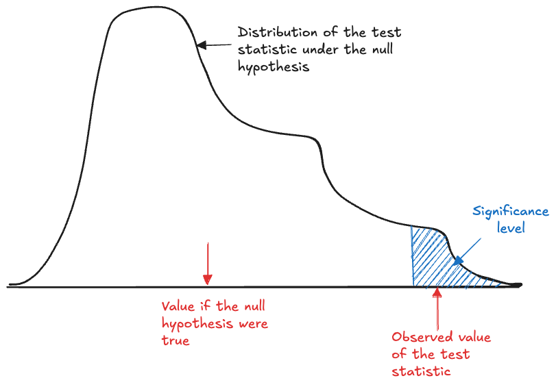
Specify a probability level \(\alpha\) that is sufficiently small that should an event occur with this probability (or less), we discount the possibility that the event is consistent with the null hypothesis. We adopt the alternative hypothesis as a plausible explanation of the observed data instead. The level \(\alpha\) is called the significance level of the statistical test.
We compute the probability under the null hypothesis to observe a result as least as extreme as the one we obtained. This probability is called the \(p\)-value of the statistical test. If the \(p\)-value is less than the significance threshold \(\alpha\), the null hypothesis is rejected.
Computing a probability under the null hypothesis means that we consider the distribution of the test statistic assuming that the null hypothesis is true. Both decision approaches reject the null hypothesis as an explanation of the data if the observed event is highly unlikely under that distribution.
The difference in the two approaches is whether we decide on the null hypothesis based on comparing the value of the statistic to the rejection region under the null hypothesis or based on the \(p\)-value. The rejection region is the area under the null distribution that covers \(\alpha\) probability. If the alternative is one-sided, the rejection region is in one tail of the distribution. If the alternative is two-sided, the rejection region can fall in separate tails of the distribution. (Some tests are implicitly two-sided and have a single rejection region, for example, \(F\) tests).
If you reject a test at the significance level \(\alpha\) then you reject the test for all \(p\)-values less than \(\alpha\).
Figure 60.17 shows the \(p\)-value for a one-sided test where the test statistic takes on larger value if the null hypothesis is not true. The \(p\)-value corresponds to the shaded area, the probability of observing values of the test statistic a least as extreme as what we got. If the test would be two-sided and the test statistic would be inconsistent with \(H\) for small values as well, a second region on the left side of the distribution would have to be considered.
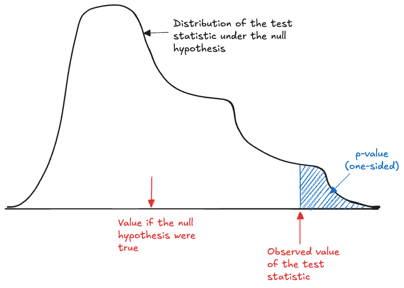
Figure 60.18 shows the decision procedure when we work with the significance level \(\alpha\). The shaded region in the tail of the null distribution is the rejection region for this one-sided test. The area under the density of the region is exactly \(\alpha\). If the test statistic falls into this region, the null hypothesis is rejected.
Returning to the previous example of testing \(H:\pi = 0.75\) against \(H_a:\pi > 0.75\), recall that by the CLT and under the null hypothesis \(\widehat{\pi} \sim G(0.75,0.75\times 0.25/n)\). The probability to observe a particular sample proportion (or a more extreme result) under the null hypothesis is a function of \(n\), since the variance of the sample statistic depends on \(n\).
If the null hypothesis is very wrong then it should be easy to reject \(H\) based on a small sample size; the test statistic will be far in the tail of the null distribution. If the null hypothesis is only a bit wrong, we can still reject \(H\) when \(n\) is sufficiently large, because we can control the variance of \(\widehat{\pi}\) through the sample size. In other words, we can affect the dispersion of the null distribution through \(n\) and create a situation where even tiny deviations from the value under the null hypothesis are significant.
These considerations lead to an important point: there is a difference between statistical significance and practical importance. Just because a result is statistically significant—that is, it is not consistent with a null hypothesis, does not imply that we care about the magnitude of the detected difference. Suppose you compare two fertilizer treatments and reject the hypothesis that they produce the same crop yield per acre (\(H:\mu_1 = \mu_2\)). The observed difference between the yields is 0.0025 bushels per acre. While statistically significant, it is not practically relevant and nobody would launch a marketing campaign to promote the fertilizer with the slightly higher yield. If, however, the statistical significant difference is 25 bushels/acre we feel much different about it.
Conclusions
The conclusion of a statistical test is whether the null hypothesis can be rejected or is failed to be rejected. We never know whether the alternative hypothesis is true. If we knew that ahead of time there would be no statistical problem.
The test is performed under the assumption that \(H\) is true and the best we can do is reject or not reject that hypothesis. Failing to reject the null hypothesis does not make it true. We only assumed that it was true for the purpose of calculating probabilities. You should avoid statements such as “We accept the null hypothesis”.
Statistical errors
Statistical decisions are based on probabilities of events and so are inherently uncertain and possibly wrong. A null hypothesis is rejected when the likelihood of a result as extreme as the one observed is less than \(\alpha\). In \(\alpha\times 100\%\) of such rejections we are making a mistake: rejecting a true null hypothesis. Similarly, if the null hypothesis is not true we might erroneously fail to reject it, if the data is not sufficiently disagreeable with the null hypothesis.
These two errors are called the Type I and Type II errors, or the errors of the first and second kind. In case of a confusion matrix where a positive result corresponds to rejection of the null hypothesis, a Type I error is a false positive and a Type II error is a false negative (Table 60.3).
| Decision about \(H\) | \(H\) is true | \(H\) is not true |
|---|---|---|
| Do not reject | Correct (\(\Pr = 1-\alpha\)) | Type II Error (\(\Pr =\beta\)) |
| Reject | Type I Error (\(\Pr = \alpha\)) | Correct (\(\Pr = 1-\beta\)) |
| Decision about \(H\) | \(H\) is true | \(H\) is not true |
|---|---|---|
| Do not reject | True Negative (\(\Pr = 1-\alpha\)) | False Negative (\(\Pr =\beta\)) |
| Reject | False Positive (\(\Pr = \alpha\)) | True Positive (\(\Pr = 1-\beta\)) |
\(\alpha\) and \(1-\alpha\) are complement probabilities under the null distribution, the distribution of the test statistic if \(H\) is true. \(\beta\) and \(1-\beta\) are probabilities under a different distribution, the alternative distribution. In a test that specifies the alternative hypothesis as a range, for example, \(H_a: \mu > 5\), all values greater than 5 are consistent with the alternative, and the beta probabilities depend on the value under \(H_a\). Figure 60.19 displays this idea with three distributions of the test statistic: the distribution under the null hypothesis and two possible distributions under the alternative. The Type II error is the probability under the alternative distribution to the left of the decision criterion, the direction in which the null is not rejected.
The correct decision in the lower right corner of Table 60.3, to correctly reject a null hypothesis that is not true, is the decision we would like to make. The associated probability \(1-\beta\) is known as the power of the test.
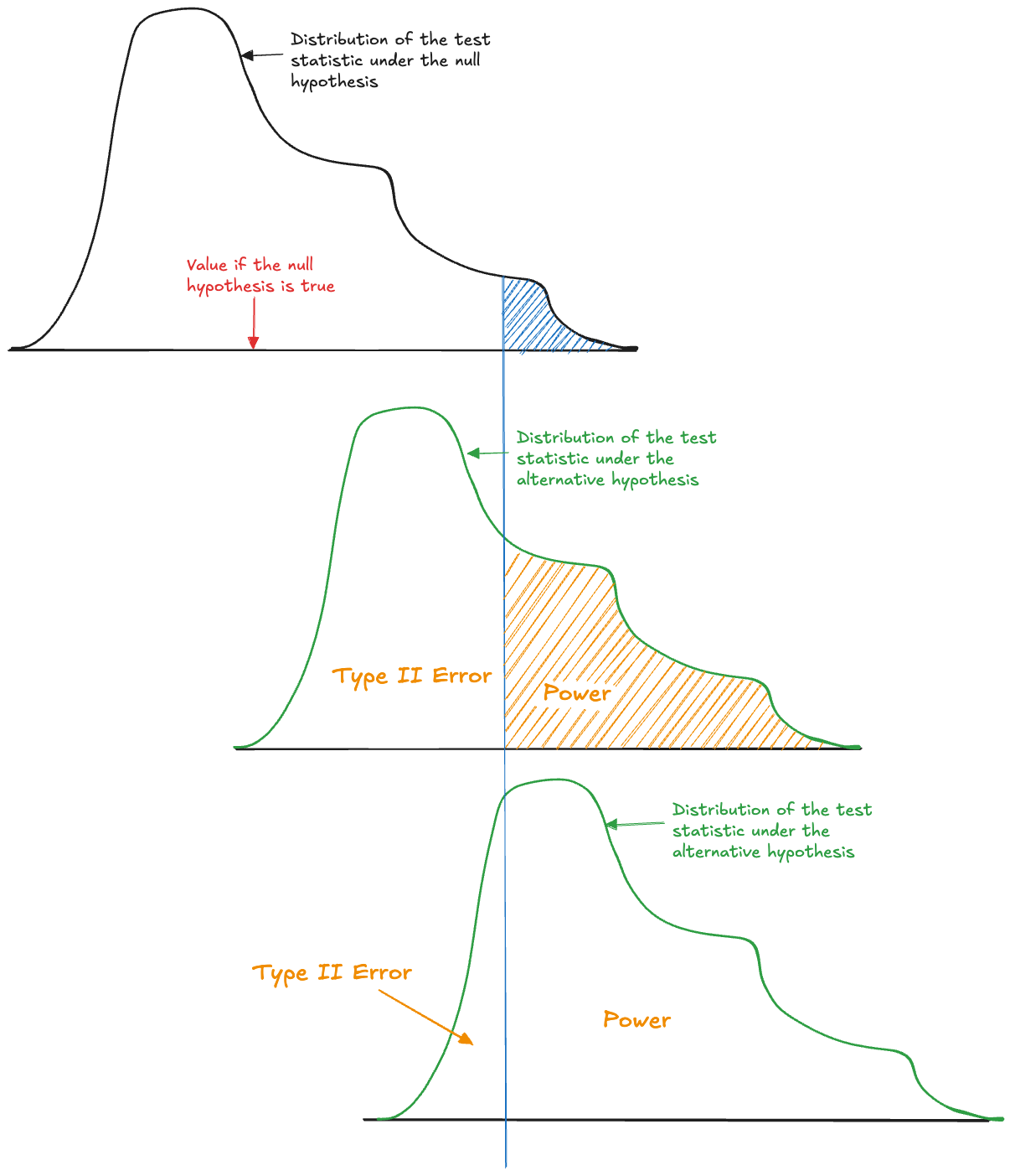
As the alternative distribution in Figure 60.19 moves further to the right—the null hypothesis becomes more wrong—the power of the test increases. While it is desirable to have large power, because we want to reject an incorrect null with high probability, the power can be manipulated. Simply specify a null hypothesis that is very wrong, and you will increase the probability to detect that. The distribution of the test statistic typically depends on the size of the experiment (the sample size \(n\)). By observing more data the power of a test increases. The difference between statistical significance and practical relevance comes to the fore here. With large sample sizes it is possible to overpower statistical tests to reject very small deviations from the null hypothesis that are not practically relevant.
A good study design selects a sample size to achieve a specified power to detect a difference of practical relevance.
Derivation of a Statistical Test
The derivation of a statistical test is similar to the derivation of a confidence interval. It starts with a pivot statistic for which the distribution is known if the null hypothesis is true. Depending on whether the alternative hypothesis is one- or two-sided, we then calculate the probability to observe the value of the test statistic—or a more extreme result—under \(H\). If that \(p\)-value is sufficiently small, the null hypothesis is rejected.
Example: Testing the Mean of a \(G(\mu,\sigma^2)\)
You are drawing a random sample of size \(n=15\) from a \(G(\mu,\sigma^2)\) distribution to test \(H: \mu = \mu_0 = 4\) against \(H_a: \mu \neq 4\). The observed value of the sample mean is \(\overline{y} = 5.7\) and the sample standard deviation is \(s=3.1\).
To construct a test we use as the pivot statistic \[ T = \frac{\overline{Y}-\mu}{S/\sqrt{n}} \] If the null hypothesis is true, then \[ T_0 = \frac{\overline{Y}-\mu_0}{S/\sqrt{n}} \sim t_{n-1} \] The \(p\)-value of the test is \(2\Pr(T_0 > |t_0|)\). The absolute value and the doubling of the probability is done to compute probabilities in both tail areas of the null distribution.
The value of the test statistic under the null hypothesis is \[ t_0 = \frac{5.7-4}{3.1/\sqrt{15}}=2.123 \] The probability \(2\Pr(t_{14} > 2.123) = 0.052\) is the \(p\)-value of the test.
If the significance level at which we declare that events are inconsistent (they should not have happened because they are too unlikely) is \(\alpha = 0.05\), then we would fail to reject the null hypothesis because \(p > 0.05\). If the significance level is \(\alpha = 0.1\), then we would reject \(H\).
Connection to Confidence Intervals
There is a straightforward connection between testing a hypothesis and estimating a confidence interval. Both are based on pivot statistics and quantiles of their distribution. If the observed value of the pivot—under the null hypothesis—is extreme, the null hypothesis is rejected. Similarly, the confidence interval specifies the values of the parameters that are likely supported by the data.
In other words, if you have a two-sided \((1-\alpha)\times 100\%\) confidence interval for parameter \(\theta\), then the hypothesis \(H:\theta = 0\) is rejected at the \(\alpha\) significance level for all values outside of the confidence bounds. Similarly for one-sided confidence limits and one-sided hypothesis test.
Starting with a null hypothesis \(H:\theta = \theta_0\), the hypothesis is rejected at the \(\alpha\) significance level if a corresponding \((1-\alpha)\times 100\%\) confidence interval covers \(\theta_0\).
60.6 Categorical Data
In categorical data analysis we are concerned with studying the properties of counts and proportions of categorical variables. These counts typically come from binary or multinomial distributions.
Multinomial Experiment
A multinomial experiment consists of \(n\) random samples (identical and independent trials) from a multinomial distribution with \(k\) outcomes (\(k\) categories). The categories have probabilities \(\pi_1, \pi_2, \cdots, \pi_k\) and \(\sum_{i=1}^k \pi_i = 1\). We are interested in learning about the \(n_i\), the number of sampled (trials) resulting in outcome \(i\).
Example: High Blood Pressure Clinical Trial
A clinical trial is conducted with 200 randomly chosen high blood pressure patients who receive a new drug. The patients are classified according to the following four outcomes:
- Marked decrease in blood pressure (\(i=1\))
- Moderate decrease in blood pressure (\(i=2\))
- Slight decrease in blood pressure (\(i=3\))
- No decrease or slight increase in blood pressure (\(i=4\))
The patients receive a test drug and we observe \(n_1 = 120\), \(n_2 = 60\), \(n_3=10\), and \(n_4 = 10\).
The established (standard) treatment of high blood pressure is known to lead to marked decrease in half of the patients, moderate decrease in a quarter of patients, and slight decrease in 10% of the patients.
The question is whether the outcome distribution of the new drug is different from that of the standard treatment?
The basic procedure to compare a set of categorical counts against a hypothesis is pretty straightforward:
- Make a table of the observed counts, this is called a contingency table.
- Compare a table of the expected counts, consistent with the null hypothesis.
- Compute the Pearson Chi-Square test statistic from the observed and expected counts.
- If the distributional properties of the test statistic are met, compute significance level or \(p\)-value from a reference \(\chi^2_{\nu}\) distribution.
The test statistic Karl Pearson proposed for this situation is \[ X^2 = \sum_{ij,...} \frac{\left(N_{ij,...}-E_{ij,...}\right)^2}{E_{ij,...}}=\sum_i \sum_j \cdots \frac{\left(N_{ij,...}-E_{ij,...}\right)^2}{E_{ij,...}} \]
The subscripts \({ij,...}\) denote the dimensions of the contingency table. In a one-dimensional table with \(r\) rows (or \(c\) columns), there is a single index, \[ X^2 = \sum_{i=1}^r \frac{(N_i-E_i)^2}{E_i} \] In a two-dimensional table with \(r\) rows and \(c\) columns, \[ X^2 = \sum_{i=1}^r\sum_{j=1}^c \frac{(N_{ij}-E_{ij})^2}{E_{ij}} \] \(N_{ij}\) is the observed count in row \(i\), column \(j\) of the table. \(E_{ij}\) is the expected count in row \(i\), column \(j\) that is consistent with the null hypothesis.
Example: High Blood Pressure Clinical Trial (Cont’d)
In the high blood pressure trial, the contingency table of observed counts is
| Category | \(N_i\) |
|---|---|
| Marked decrease | 120 |
| Moderate decrease | 60 |
| Slight decrease | 10 |
| No decrease or increase | 10 |
If the new blood pressure drug is equal to the standard treatment, we would expect \(H:\pi_1 = 0.5, \pi_2 = 0.25, \pi_3 = 0.1, \pi_4 = 0.15\) to hold. Based on this hypothesis we can calculate the expected counts in the four categories
| Category | \(N_i\) | \(E_i\) |
|---|---|---|
| Marked decrease | 120 | 200 x 0.50 = 100 |
| Moderate decrease | 60 | 200 x 0.25 = 50 |
| Slight decrease | 10 | 200 x 0.10 = 20 |
| No decrease or increase | 10 | 200 x 0.15 = 30 |
The Pearson test statistic is \[ X^2 = \frac{(120-100)^2}{100} + \frac{(60-50)^2}{50} + \frac{(10-20)^2}{20} + \frac{(10-30)^2}{30} = 24.33 \]
The \(\chi^2_{\nu}\) distribution is an approximation for the distribution of \(X^2\) under the null hypothesis. The approximation holds reasonably well if all expected values exceed 1 and at most 20% of the expected values are less than 5. These conditions are met in this example. Note that the criteria for the approximation are based on expected counts, not on observed counts.
The degrees of freedom of the \(\chi^2_{\nu}\) reference distribution are determined based on the number of data points that can freely be varied, generally it is the product of the table dimensions minus one. Thus, for a one-dimensional table, \(\nu = r-1\), for a two-dimensional table \(\nu = (r-1)(c-1)\) and so forth.
Tests of Homogeneity and Independece
The test of homogeneity compares multiple samples of categorical data and asks whether they have the same distribution. The test of independence is based on the cross-classification of attributes in a single sample. It turns out that the test statistic is the same for the two tests, which leads to a blurring of the lines. Often, what is described as a test of homogeneity is actually a test of independence. So where is the critical difference?
Sampling schemes
In a test of homogeneity we collect separate samples from different populations and compare the distribution of a categorical variable across the populations (across the samples). For example, collect a random sample of 200 men and ask them about their streaming platform viewing preferences. Collect a separate random sample of 200 women and ask them about their streaming platform preferences. The test of homogeneity tests the null hypothesis that the distribution of streaming platform preferences is the same among the population of men and the population of women. This sampling scheme is also known as product multinomial sampling (Fienberg (1980)).
On the other hand, if you were to collect a single sample and cross-classify the participants with respect to gender and streaming platform preferences, then you are testing a different hypothesis, because we are now discussing the relationship between two variables in a single sample. The question then is whether gender and streaming platform preference are related—the null hypothesis is whether they are independent. This is a form of multinomial sampling.
A third sampling model for contingency tables, based on the Poisson distribution, was first introduced by Fisher (1950). Without prior knowledge of the total number of observations, each cell of the table is a draw from a Poisson distribution. This sampling model is related to multinomial sampling. Take a two-dimensional table with cell counts \(N_{ij}\). If the \(N_{ij}\) are Poisson, then their conditional distribution, given the total sample size, is multinomial.
The \(r \times c\) contingency table
The difference between the two sampling schemes can be expressed in terms of the marginal totals of a 2 x 2 table. Suppose a table has \(i=1,\cdots,r\) rows and \(j=1,\cdots,c\) columns. Denote as \(N_{i.}\) the total count in row \(i\) (the marginal count of row \(i\)): \[ N_{i.} = \sum_{j=1}^c N_{ij} \] Similarly, \(N_{.j}\) is the marginal total in column \(j\), \[ N_{.j} = \sum_{i=1}^r N_{ij} \] and \(N_{..}\) is the total number of observations in the table: \[ N_{..} = \sum_{i=1}^r N_{i.} = \sum_{j=1}^c N_{.j} = \sum_{i=1}^r\sum_{j=1}^c N_{ij} \] The dot(s) in the subscript replace(s) the index over which the counts are summed.
In the product-multinomial scheme, the row totals \(N_{i.}\) are fixed by the sampling designs, they are the number of samples taken from the \(i\)th population. (If you think of columns representing populations, then the \(N_{.j}\) are fixed by the sample design). In the multinomial sampling scheme, only the overall total \(N_{..}\) is fixed (Table 60.4).
| \(j=1\) | \(j=2\) | \(\cdots\) | \(j=c\) | Margin | |
|---|---|---|---|---|---|
| \(i=1\) | \(N_{11}\) | \(N_{12}\) | \(\cdots\) | \(N_{1c}\) | \(N_{1.}\) |
| \(i=2\) | \(N_{21}\) | \(N_{22}\) | \(\cdots\) | \(N_{2c}\) | \(N_{2.}\) |
| \(\vdots\) | \(\vdots\) | \(\vdots\) | \(\ddots\) | \(\vdots\) | \(\vdots\) |
| \(i=r\) | \(N_{r1}\) | \(N_{r2}\) | \(\cdots\) | \(N_{rc}\) | \(N_{r.}\) |
| Margin | \(N_{.1}\) | \(N_{.2}\) | \(\cdots\) | \(N_{.c}\) | \(N_{..}\) |
Let \(N_{ij}\) denote the observed count in a two-dimensional contingency table such as Table 60.4. In a test of homogeneity, \(N_{ij}\) refers to the count in category \(j\) of the \(i\)th population (sample). In a test of independence, \(N_{ij}\) refers to the number of samples that fall into category \(i\) of the first variable—say gender—and category \(j\) of the second variable—say viewing preference.
The test statistic is the same in both cases: \[ X^2 = \sum_{i=1}^r \sum_{j=1}^c \frac{(N_{ij}-E_{ij})^2}{E_{ij}} \] and it has a \(\chi^2_{(r-1)(c-1)}\) distribution under the null hypothesis. The expected counts in row \(i\), column \(j\) of the table are calculated as \[ E_{ij} = \frac{N_{i.}N_{.j}}{N_{..}} \]
How did we arrive at this expression for \(E_{ij}\)? Suppose the two columns of the table represent variables \(X\) and \(Y\). Under the multinomial and product-multinomial sampling models, each cell of the table is backed by a probability \(\pi_{ij}\), which can be estimated as \[ \widehat{\pi}_{ij} = N_{ij}/N_{..} \] Also, the margins are backed by marginal probabilities \(\pi_{i.}\) and \(\pi_{.j}\)
If \(X\) and \(Y\) are independent, they are not associated with each other, and the cell probability \(\pi_{ij}\) can be calculated based on the marginal probabilities \[ \Pr(X=x_i,Y=y_j) = \Pr(X=x_i)\Pr(Y=y_j) = \pi_{i.}\times\pi_{.j} \] This leads to a different estimator \[ \tilde{\pi}_{ij} = \widehat{\pi}_{i.} \times \widehat{\pi}_{.j} = \frac{N_{i.}}{N_{..}} \times \frac{N_{.j}}{N_{..}} \] The expected cell frequency under independence follows as \[ E_{ij} = N_{..} \times \tilde{\pi}_{ij} = \frac{N_{i.}N_{.j}}{N_{..}} \]
How do you explain the degrees of freedom \(\chi^2_{(r-1)(c-1)}\) of \(X^2\)? In order to maintain the margins and the overall total in the table, how many cell values can you choose freely? For each of the \(r-1\) rows you can choose \(c-1\) values independently. The \(c\)th value in each row and the \(r\)th value in each column are then determined, otherwise the marginal totals cannot be achieved.
Measures of Association
The primary measure of association for continuous variables is the Pearson product-moment correlation coefficient. Other measures, such as the robust Kendall’s \(\tau\) or Spearman’s \(\rho\) statistics are also in use—these are based on ranks of the continuous outcomes.
But, how do you measure association between two qualitative variables?
Let’s consider the simple case of a 2x2 table cross-classifying categorical variables \(X\) and \(Y\) (Table 60.5).
| \(Y_1\) | \(Y_2\) | Margin | |
|---|---|---|---|
| \(X_1\) | \(N_{11}\) | \(N_{12}\) | \(N_{1.}\) |
| \(X_2\) | \(N_{21}\) | \(N_{22}\) | \(N_{2.}\) |
| Margin | \(N_{.1}\) | \(N_{.2}\) | \(N_{..}\) |
Odds ratio
The estimate of the cell probability \(\pi_{ij}\), without imposing any hypothesis, is \(\widehat{\pi}_{ij} = N_{ij}/N_{..}\).
The odds of an event is defined as the ratio of the event probability and its complement. For example, the odds of \(Y_1\) in the presence of \(X\) are \[ O_{y_1} = \frac{\pi_{11}}{\pi_{21}} \] The odds of \(Y_2\) in the presence of \(X\) are \[ O_{y_2} = \frac{\pi_{12}}{\pi_{22}} \]
Similarly, we can define odds of \(X\) in the presence of \(Y\): \[ O_{x_1} = \frac{\pi_{11}}{\pi_{12}} \qquad O_{x_2} = \frac{\pi_{21}}{\pi_{22}} \]
The odds specify how likely one event is relative to another. The odds ratio, also known as the cross-product ratio, relates those odds to each other: \[ OR = \frac{O_{x_1}}{O_{x_2}} = \frac{\pi_{11}/\pi_{12}}{\pi_{21}/\pi_{22}} = \frac{\pi_{11}\pi_{22}}{\pi_{21}\pi_{12}} \] The log odds ratio is the log off this expression: \[ \log(OR) = \log(\pi_{11})+\log({\pi_{22}}) - \log(\pi_{21}) - \log({\pi_{12}}) \]
The odds ratio has nice properties.
Interpretation. If \(OR > 1\), then \(X\) and \(Y\) are associated (correlated) in the sense that, compared to the absence of \(X\), the presence of \(X\) raises the odds of \(Y\), and symmetrically the presence of \(Y\) raises the odds of \(X\). If \(OR < 1\), then \(X\) and \(Y\) have a negative association, the presence of one reduces the odds of the other.
Test for independence. \(X\) and \(Y\) are independent if their odds ratio is one (log odds ratio is zero). The odds of one event then do not change due to the presence or absence of the other variable.
Symmetry. Computing the odds ratio by relating the odds of \(Y\) yields \[ OR = \frac{O_{y_1}}{O_{y_2}} = \frac{\pi_{11}/\pi_{21}}{\pi_{12}/\pi_{22}} = \frac{\pi_{11}\pi_{22}}{\pi_{21}\pi_{12}} \]
Invariance under permutation If you change the order of the rows, (the order of the columns), the log odds ratio changes sign. If you exchange \(X_1\) and \(X_2\), then \[ O_{x_1} = \frac{\pi_{21}}{\pi_{22}} \qquad O_{x_2} = \frac{\pi_{11}}{\pi_{12}} \] and \[ OR = \frac{\pi_{21}/\pi_{22}}{\pi_{11}/\pi_{12}} = \frac{\pi_{21}\pi_{12}}{\pi_{11}\pi_{22}} \] which is the reciprocal of the odds ratio calculated earlier.
Statistical tests and confidence intervals for the odds ratio are based on the asymptotic distribution of the log odds ratio. The estimated log odds ratio has an approximate Gaussian distribution with mean \(\log(OR)\) and variance \[ \frac{1}{N_{11}} + \frac{1}{N_{12}} + \frac{1}{N_{21}} + \frac{1}{N_{22}} \]
Cramer’s \(V\)
The \(V\) statistic of Cramer is a general measure of association for \(r \times c\) contingency tables. It is based on the Pearson statistic and given by \[ V = \sqrt{\frac{X^2}{N_{..}\times \min\{(r-1),(c-1)\}}} \] \(V\) falls between 0 and 1, with 0 indicating that the row and column variable of the contingency table are not related.
Measures of Agreement
When the rows and columns of a contingency table refer to the same variable, observed under different conditions or measured in different ways, then we expect them not to be independent. For example, if two teaching assistants grade the same set of papers, we do not expect them to be unrelated. We expect there to be some agreement between the grades. When we compare the target values in the test data set of a binary classification with the predicted categories from a statistical model, we do not expect observed and predicted categories to be unrelated; we expect some agreement.
| 1 | 2 | 3 | 4 | 5 | Margin | |
|---|---|---|---|---|---|---|
| 1 | 10 | 6 | 4 | 2 | 2 | 24 |
| 2 | 12 | 20 | 16 | 7 | 2 | 57 |
| 3 | 1 | 12 | 30 | 20 | 6 | 69 |
| 4 | 4 | 5 | 10 | 25 | 12 | 56 |
| 5 | 1 | 3 | 3 | 8 | 15 | 30 |
| Margin | 28 | 46 | 63 | 62 | 37 | 236 |
Agreement and association are two forms of structured interaction between two variables. Agreement is based on the concordance between the rows and columns of a table; the values that fall on the diagonal versus the values in off-diagonal cells. The computations based on a 2 x 2 confusion matrix are a special case (Section 23.3.3.3).
The appropriate measure of agreement depends on the nature of the data and the size of the table. Table 60.6 displays the data for two raters who evaluated the quality of 236 experimental units from 1–5. The result is a 5 x 5 table with ordinal rows and columns. The order of the rows and columns is relevant.
Cohen’s Kappa (\(\kappa\))
Cohen’s \(\kappa\) statistic measures the agreement between two raters in a square table (\(r \times r\)). It is based on the simple idea to adjust the observed degree of agreement for the amount of agreement the two raters would have exhibited purely by chance. \(\kappa\) is suitable for nominal (unordered) categories; a weighted form of the Kappa statistic is available for ordered categories.
Let \(\pi_{ij}\) denote the probability for a rating in category \(i\) by the first rater and a rating in category \(j\) by the second rater. The observed level of agreement between the ratings is obtained from the diagonal cells: \[ \pi_o = \sum_{i=1}^r \pi_{ii} \] If the ratings are independent, we do not expect zero agreement. Some counts would fall on the diagonal by chance. This chance agreement can be calculated from the marginal probabilities: \[ \pi_e = \sum_{i=1}^r \pi_{i.}\pi_{.j} \]
The Kappa statistic is defined as \[ \kappa = \frac{\pi_o - \pi_e}{1-\pi_e} = 1 - \frac{1-\pi_o}{1-\pi_e} \]
Complete agreement results in \(\kappa = 1\). If the rater agreement is no greater than what would be expected by chance, then \(\kappa=0\). The theoretical maximum value of 1 requires that the row and column totals are identical. For any given table, the maximum achievable value of \(\kappa\) is \[ \kappa_{\text{max}} = \frac{-\pi_e + \sum_{i=1}^r\min\{\pi_{i.},\pi_{.j}\}}{1-\pi_e} \]
For a 2 x 2 table such as the confusion matrix of a binary classification model, \(\kappa\) can be expressed in terms of the true positive, true negative, false positive, and false negative counts: \[ \kappa = \frac{2(TP\times TN - FN \times FP)}{(TP + FP) \times (FP+TN) + (TP+FN) \times (FN+TN)} \]
60.7 Simple Linear Regression
A regression model is a statistical model that describes how the mean of a random variable—called the target, response, output, or dependent variable—changes with the values of other variables—called the input, regressor, predictor, or independent variables.
The name regression dates back to Francis Galton who examined in the 19th century the relationship between the heights of fathers and the heights of sons. He noticed that taller fathers have taller sons than shorter fathers, but that sons of tall fathers tend to be shorter and sons of short fathers tend to be taller than their fathers. Galton considered this phenomenon a regression to “mediocrity”. Today we call it a regression to the mean. The term regression to describe statistical relationships between variables persists to this day.
The simplest regression model is that between a continuous target variable \(Y\) and a continuous input variable \(X\). If the relationship were deterministic (functional), it could be written as \[ Y = f(x) \] Furthermore, if the relationship is linear, it can be written as \[ Y = \beta_0 + \beta_1 x \tag{60.8}\]
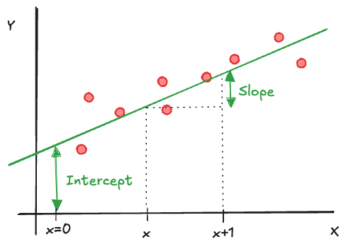
The parameters of this relationship are the intercept \(\beta_0\) and the slope \(\beta_1\). \(\beta_0\) represents the value of \(Y\) when \(x=0\), \(\beta_1\) is the change in \(Y\) if \(x\) increases by one unit: \[ f(x+1) - f(x) = \beta_0 + \beta_1(x+1) - \beta_0 - \beta_1 x = \beta_1 \]
A statistical relationship allows for variation of the response at a given value \(x\), in other words, we are dealing with distributions \(p(Y|x)\), one for each possible value of \(X\). Model Equation 60.8 becomes a statistical model by adding a random element, the model errors \(\epsilon\) (Figure 60.20): \[ Y = \beta_0 + \beta_1 x + \epsilon \]
The observational form of the model adds subscripts to identify the observations in a particular sample: \[ Y_i = \beta_0 + \beta_1 x_i + \epsilon_i \qquad i=1,\cdots,n \]
The stochastic properties of \(Y_i\) are induced by the properties of \(\epsilon_i\). The customary assumptions for the error process are
- The errors have zero mean: \(\text{E}[\epsilon_i] = 0, \forall i\).
- The errors have equal variance (homoscedasticity): \(\text{Var}[\epsilon_i] = \sigma^2, \forall i\).
- The errors are uncorrelated: \(\text{Cov}[\epsilon_i,\epsilon_j] = 0, \forall i,j, i\ne j\).
Under these error conditions it is easy to show that
\[\begin{align*} \text{E}[Y_i] &= \beta_0 + \beta_1 x_i \\ \text{Var}[Y_i] &= \sigma^2, \quad\forall i \\ \text{Cov}[Y_i, Y_j] &= 0, \quad\forall i,j, i \ne j \end{align*}\]
The regression model expresses how the mean (expected value) of the random variable \(Y\) changes functionally with \(X\) and the amount of variability around that mean (\(\sigma^2\)).
The nine observed values in Figure 60.20 do not fall on the regression line, they scatter about it. At each value of \(x\), the observed value of \(Y\) is the realization of a random draw from a distribution with mean \(\text{E}[\epsilon] = 0\) and variance \(\text{Var}[\epsilon] = \sigma^2\). If we were to repeat the sample process with the same set of \(x\) values, we would get a different set of nine points; the overall scatterplot would look similar, but the placement of the points along the \(Y\) axis would be different. How, then, can we estimate the parameters \(\beta_0\) and \(\beta_1\) of the mean function and the variance \(\sigma^2\) of the error process based on a single sample of nine points?
Ordinary Least Squares Estimation
The intercept \(\beta_0\) and \(\beta_1\) are commonly estimated by least squares. The principle of least squares estimation can be approached from several viewpoints, for example in terms of geometry or as a function minimization problem. More on this in Section 62.2. Here we provide a simple geometric interpretation.
The line in Figure 60.20 represents the true mean function \(\beta_0 + \beta_1x\); it is unknown. Our example regression problem starts with a set of nine data pairs \((Y_i,x_i), i=1,\cdots,9\) as shown in Figure 60.21.
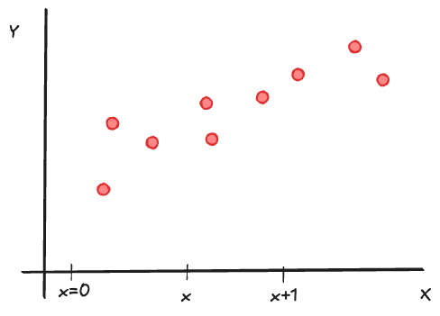
How should we fit a line to these data points? There are many candidates corresponding to different pairs \((\beta_0^*,\beta_1^*)\) and we need to somehow choose the “best” pair of values (Figure 60.22).
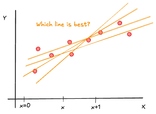
Sums of squares
To do this we first need to define what “best” means in this situation. The least squares principle states to choose those values \((\widehat{\beta}_0, \widehat{\beta}_1)\) that minimize the sum of the squared deviations between the observed values and the fitted line (Figure 60.23). Imagine placing a square at each data point, with its side parallel to the \(Y\)-axis. That is, we are measuring distance perpendicular to the \(x\)-axis and not perpendicular to the regression line. Square those distances to get the area of each of the squares.
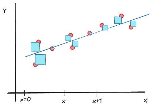
Summing the areas of the squares across the data set (here, nine points), yields a sum of squares. Because the distance between an observation \(y_i\) and its point on the regression line \(y_i^*\) is called a residual, the sum of squares in question is the residual sum of squares (SSR, also called the error sum of squares, SSE) \[ \text{SSE} = \sum_{i=1}^n \left(y_i - y_i^*\right)^2 = \sum_{i=1}^n \left(y_i - \beta_0^* - \beta_1^* x_i\right)^2 \tag{60.9}\]
This notation seems odd, why introduce “star” notation? Every pair of values \((\beta_0^*, \beta_1^*)\) results in predicted values \(y_i^*\), residuals \(y_i - y_i^*\) and an error sum of squares. The estimation principle is to choose as the least squares solution the values that minimize SSE. We call those specific values the least squares estimates \(\widehat{\beta}_0\) and \(\widehat{\beta}_1\). More precisely, because the error conditions above are referred to as the ordinary error properties (equal variance, no correlations), the procedure is known as ordinary least squares (OLS) estimation.
Important
Squaring the deviations between observed and predicted values makes sense to ensure that positive and negative deviations from the line do not cancel each other out. This leads naturally to a least squares criterion for estimation. Other criteria are possible. For example, we could choose estimators that minimize \[ \sum_{i=1}^n |y_i - y_i^*| \] the sum of absolute deviations. This is known as least absolute deviation (LAD) or least absolute error (LAE) regression. The solutions are different from the least squares estimates.
Working with the squared deviations is mathematically convenient and the least squares estimators have very nice statistical properties. Absolute deviations have the advantage of robustness against outlying observations. Extreme values of \(Y\) affect squared differences more than absolute differences. LAD is used as a robust method of regression estimation when outliers are present.
Normal equations
To minimize SSE, we can take derivatives of Equation 60.9 with respect to \(\beta_0^*\) and \(\beta_1^*\), set them to zero and solve. This leads to two equations, called the normal equations. Since we are now solving for the specific least squares solution, we re-introduce the hat notation:
\[\begin{align*} \sum_{i=1}^n y_i = n \widehat{\beta}_0 + \widehat{\beta}_1 \sum_{i=1}^n x_i \\ \sum_{i=1}^n x_i y_i = \widehat{\beta}_0\sum_{i=1}^n x_i + \widehat{\beta}_1\sum_{i=1}^n x_i^2 \end{align*}\]
Solving the equations leads to the following formulas for the OLS estimates:
\[\begin{align*} \widehat{\beta}_1 &= \frac{\sum_{i=1}^n(x_i-\overline{x})(y_i-\overline{y})}{\sum_{i=1}^n(x_i-\overline{x})^2}\\ \widehat{\beta}_0 &= \overline{y} - \widehat{\beta}_1 \overline{x} \end{align*}\]
If we want to emphasize the OLS estimators, we use the random variable (uppercase) notation for \(Y\):
\[\begin{align*} \widehat{\beta}_1 &= \frac{\sum_{i=1}^n(x_i-\overline{x})(Y_i-\overline{Y})}{\sum_{i=1}^n(x_i-\overline{x})^2}\\ \widehat{\beta}_0 &= \overline{Y} - \widehat{\beta}_1 \overline{x} \end{align*}\]
This also highlights that we consider in regression models the \(X\) values as constants, not the realization of random variables.
OLS properties
If the ordinary error conditions hold, the OLS estimators have the following properties:
- \(\widehat{\beta}_0\) is unbiased for \(\beta_0\): \(\text{E}[\widehat{\beta}_0] = \beta_0\).
- \(\widehat{\beta}_1\) is unbiased for \(\beta_1\): \(\text{E}[\widehat{\beta}_1] = \beta_1\).
- The sum of the residuals is zero: \(\sum_{i=1}^n (y_i - \widehat{y}_i) = 0\).
- The sum of the observed values is equal to the sum of the fitted values: \(\sum_{i=1}^n y_i = \sum_{i=1}^n \widehat{y}_i\).
- The average fitted value is the sample mean (follows from 4.): \(\frac{1}{n}\sum_{i=1}^n \widehat{y}_i = \overline{y}\).
- The fitted line passes through the point \((\overline{x},\overline{y})\).
- The inner product of residuals and fitted values is zero (they are orthogonal): \(\sum_{i=1}^n \widehat{y}_i(y_i - \widehat{y}_i) = 0\).
- The inner product of residuals and \(X\) values is zero (they are orthogonal): \(\sum_{i=1}^n x_i(y_i - \widehat{y}_i) = 0\).
You can show these properties based on the normal equations—give it a try.
Estimating \(\sigma^2\)
Estimating the variance of the model errors is not part of the least squares solution. In fact, the formulas for \(\widehat{\beta}_0\) and \(\widehat{\beta}_1\) do not involve \(\sigma^2\) at all. In ordinary least squares estimation, the variability of the model errors does not affect the point estimators of intercept and slope(s); it affects the precision of these estimators.
We thus need an estimate of \(\sigma^2\) if we want to measure the uncertainty in the estimators, in predicted values, if we want to test hypotheses, or calculate confidence intervals.
The typical estimator of the error variance is based on the least squares SSE, \[ \widehat{\sigma}^2 = \frac{\text{SSE}}{n-1} = \frac{\sum_{i=1}^n(y_i - \widehat{y}_i)^2}{n-1} \] This estimator is unbiased for \(\sigma^2\).
Inference About \(\beta_1\)
The slope is more important in statistical investigations than the intercept of the regression model. The slope measures the change in the mean of \(Y\) for a unit change in \(X\). If the slope is zero, the target variable does not depend on the input variable—there is no relationship.
About the intercept
The intercept, on the other hand, is rarely the subject of hypothesis tests. An exception might be a situation where \(x=0\) is a meaningful value. If \(X\) is the amount of fertilizer applied, \(x=0\) corresponds to no fertilizer application and \(\beta_0\) represents a baseline outcome. We include the intercept in the model because a model without an intercept does not make sense (would \(x=0\) imply that \(\text{E}[Y]=0\)?), not because it is of importance for research questions.
Because the \(X\) are considered fixed in a regression model, it is easy to show that the variance of the OLS slope estimator is \[ \text{Var}[\widehat{\beta}_1] = \frac{\sigma^2}{\sum_{i=1}^n(x_i - \overline{x})^2} \] To estimate this variance we replace \(\sigma^2\) with its estimate:
\[ \widehat{\text{Var}}[\widehat{\beta}_1] = \frac{\widehat{\sigma}^2}{\sum_{i=1}^n(x_i - \overline{x})^2} \]
The square root of this expression is the standard error of the slope estimator \[ \text{se}[\widehat{\beta}_1] = \sqrt{\frac{\widehat{\sigma}^2}{\sum_{i=1}^n(x_i - \overline{x})^2}} \]
If the model errors are Gaussian distributed, in addition to the error conditions listed previously, then by the linearity property of Gaussian random variables, the \(Y_i\) are also Gaussian distributed, and so are the OLS estimators. It then follows that the pivot statistic \[ T = \frac{\widehat{\beta}_1 - \beta_1}{\text{se}[\widehat{\beta}_1]} \] follows a \(t_{n-2}\) distribution. A \((1-\alpha)\times 100\%\) confidence interval for the slope is \[ [\widehat{\beta}_1 \pm t_{\alpha/2,n-2}\times\text{se}[\widehat{\beta}_1]] \] It is noteworthy that the degrees of freedom of the pivot distribution are \(n-2\). In Section 60.4.2 we constructed a \(t\)-based confidence interval for the mean of a Gaussian distribution and it had \(n-1\) degrees of freedom. Where did we lose a degree of freedom in the regression model? The reference distribution is \(t_{n-2}\) because we estimated two parameters to determine the mean function: \(\beta_0\) and \(\beta_1\).
Prediction and Confidence Intervals
The value \(\widehat{y}_i\) is called a predicted value, it is obtained by evaluating the regression model at the parameter estimates: \[ \widehat{y}_i = \widehat{\beta}_0 + \widehat{\beta}_1 x_i \]
If we refer to any value of \(x\), not necessarily one represented in the sample, we use the notation \(x_0\). This can be an observed value (one of the \(x_i\)s), a new value within the observed range of \(Xs\) (between \(\min\{x\}\) and \(\max\{x\}\)) or a value outside the range. The predicted value is then simply
\[ \widehat{y}_0 = \widehat{\beta}_0 + \widehat{\beta}_1 x_0 \tag{60.10}\]
Caution
Do not confuse the zero subscript notation on \(y\) and \(x\) and the intercept. \(\widehat{y}_0\) refers to a predicted value at an arbitrary value \(x_0\), \(\beta_0\) refers to the intercept of the model.
This seems clear cut, but there is a wrinkle. \(\beta_0 + \beta_1x_0\) is the mean of \(Y_0\), the random variable is \(\beta_0 + \beta_1 x_0 + \epsilon_0\): \[\begin{align*} Y_0 & = \beta_0 + \beta_1 x_0 + \epsilon_i \\ \text{E}[Y_0] &= \beta_0 + \beta_1 x_0 \end{align*}\]
What is Equation 60.10 estimating? And does it make a difference? We cannot observe \(\epsilon_0\) because we do not know the true values \(\beta_0\) and \(\beta_1\). If we were to estimate \(\epsilon_0\), the most plausible value would be zero, since \(\epsilon_0 \sim (0,\sigma^2)\).
The upshot is that whether we want to predict \(Y_0\) or \(\text{E}[Y_0]\), we use the same value: \(\widehat{y}_0 = \widehat{\beta}_0 + \widehat{\beta}_1 x_0\).
OK, great. So why making a big deal out of it?
- Because it is easy to forget which quantity we wish to predict when the formulas are the same.
- Because the variability of the two predictions is different.
If we predict the mean of the observations, \(\text{E}[Y_0]\), then \[ \text{se}[\widehat{Y}_0] = \sqrt{\widehat{\sigma}^2\left[\frac{1}{n} + \frac{(x_0 - \overline{x})^2}{\sum_{i=1}^n(x_i-\overline{x})^2}\right]} \tag{60.11}\]
If we predict an individual observation, then \[ \text{se}[\widehat{Y}_0] = \sqrt{\widehat{\sigma}^2\left[1 + \frac{1}{n} + \frac{(x_0 - \overline{x})^2}{\sum_{i=1}^n(x_i-\overline{x})^2}\right]} \tag{60.12}\]
The difference between Equation 60.11 and Equation 60.12 is subtle; the term \(1+\) under the square root. The term is present in the standard error expression for the individual prediction because we need to account for the inherent variability in the data when drawing a new observation—we gained an additional \(\sigma^2\). In practice, this small mathematical difference makes a huge difference numerically (Figure 60.24).
Another interesting aspect of Equation 60.11 and Equation 60.12 is the term under the square root that depends on \(x\), specifically \((x_0 - \overline{x})^2\). The further the prediction location \(x_0\) is from the center \(\overline{x}\) of the input data, the larger the standard error. Prediction and confidence intervals are most narrow at \(x_0 = \overline{x}\), and increase as you move away from the center. Predicting outside of the observed range of the input variable comes with a lot of uncertainty (Figure 60.24).
Confidence intervals for random variables are called prediction intervals. When attaching a measure of uncertainty to a predicted value, we need to be clear whether we intend to predict the mean or an individual observation. A prediction interval for \(Y_0\) is considerably wider than a confidence interval for \(\text{E}[Y_0]\).
Confidence Interval for \(\text{E}[Y_0]\) \[ \widehat{y}_0 \pm t_{\alpha/2,n-2} \sqrt{\widehat{\sigma}^2\left[\frac{1}{n} + \frac{(x_0 - \overline{x})^2}{\sum_{i=1}^n(x_i-\overline{x})^2}\right]} \]
Prediction Interval for \(Y_0\) \[ \widehat{y}_0 \pm t_{\alpha/2,n-2} \sqrt{\widehat{\sigma}^2\left[1 + \frac{1}{n} + \frac{(x_0 - \overline{x})^2}{\sum_{i=1}^n(x_i-\overline{x})^2}\right]} \]
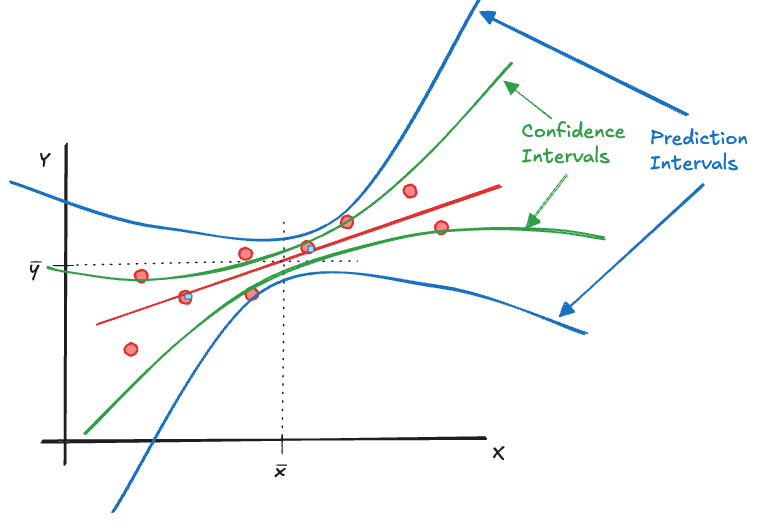
In summary, whether we predict the constant \(\text{E}[Y_0]\) or the random variable \(Y_0\) is not reflected in the point estimate, but in the variability of the point estimate.
60.8 Simple Logistic Regression
Setup
The simple linear regression (SLR) model has a continuous input variable and a single input variable. The statistical model is written as a model with additive error terms that have zero mean, equal variance, and are uncorrelated:
\[\begin{align*} Y_i & = \beta_0 + \beta_1 x_i + \epsilon\\ \text{E}[\epsilon_i] &= 0 \quad \forall i=1,\cdots,n\\ \text{Var}[\epsilon_i] &= \sigma^2 \quad \forall i=1,\cdots,n \\ \text{Cov}[\epsilon_i,\epsilon_j] &= 0, \quad \forall i,j, i\ne j \end{align*}\]
The parameters of the SLR model are estimated by ordinary least squares, minimizing the sum of squared errors, \(\text{SSE} = \sum_{i=1}^n (y_i - \widehat{y}_i)^2\).
If the target variable \(Y\) is binary instead of continuous, and takes on the values 1 (for an event) and 0 (for a non-event), the SLR model does not apply. It breaks down in a number of ways:
We know that the target variable follows a Bernoulli distribution with parameter \(\pi\), the probability to observe an event. A regression models the mean as a function of inputs. We have to relate the input(s) to a probability in a meaningful way.
A linear model for the mean does not make sense, there is no guarantee that the predictions from \(\beta_0 + \beta_1 x\) are between 0 and 1, as required for a probability.
The variance of the observations is not constant, since for a Bernoulli(\(\pi\)) random variable \(\text{Var}[Y] = \pi(1-\pi)\). As the mean changes, the variability changes.
The model for \(Y_i\) cannot be written with an additive error term with zero mean and constant variance.
Measuring the discrepancy between observed values and predicted values as squared differences does not make sense when the observed values are only zeros and ones. A different objective function than SSE is needed to judge the quality of estimators.
Figure 60.25 shows data from a credit default data set with a binary outcome, whether an account holder defaulted on a credit card, and two input variables: the account holder’s income and student status (No, Yes). Suppose we want to model the probability of credit card default as a function of income. Drawing a straight line through these data makes no sense. Instead, the model should approach 0 and 1 but not cross the values, this suggests some form of a nonlinear relationship between probability of credit card default and income.

Logistic regression is a popular method to model how probabilities in binary data change with input variables. Like SLR, simple logistic regression has a single input variable. But it differs from SLR in important ways:
A transformation of the mean is linearly related to the input variable. The transformation ensures that predictions of the mean do not fall outside of the allowable range. The transformation is invertible so that we can switch easily between making statements about \(\text{E}[Y]\) and \(\beta_1\).
Because we know the distribution of the data, estimation is based on the maximum likelihood principle, and not least squares. More on maximum likelihood estimation in Section 62.4.
Link Function
Logistic regression derives its name from the transformation referred to in 1. The transformation is known as the logit and its inverse is the c.d.f. of the standard logistic distribution function.
\[\begin{align*} \text{logit}\{\pi\} &= \log\left\{\frac{\pi}{1-\pi}\right\} = \beta_0 + \beta_1 x \\ \pi &= \frac{1}{1+\exp\{-\beta_0 - \beta_1 x\}} \end{align*}\]
The logit function is called the link function of the model, it maps the mean to the real line. The inverse link function, maps the linear predictor \(\beta_0 + \beta_1 x\) from the real line to the \((0,1)\) interval. Other functions than the logit can be used as the link function; any c.d.f. of a continuous distribution can serve as the inverse link function.
Maximum Likelihood Estimation
The maximum likelihood principle asks to use as estimators those values that maximize the likelihood function. The likelihood function is mathematically the joint distribution of the data, but we consider it a function of the parameters given the data, rather than the other way around.
For sample of \(n\) Bernoulli(\(\pi\)) random variables, the likelihood function is \[ \prod_{i=1}^n \, \pi^{y_i} \, (1-\pi)^{1-y_i} \]
For the logistic regression setup this needs to be modified since the event probability changes from observation to observation: \[ \prod_{i=1}^n \, \pi_i^{y_i} \, (1-\pi_i)^{1-y_i} \] where \(\pi_i = (1+\exp\{-\beta_0 - \beta_1 x_i\})^{-1}\).
Because the values that maximize the likelihood also maximize the log likelihood, and it is easier to work with sums rather than products, we express the estimation problem as maximizing the log likelihood (or minimizing the negative log likelihood):
\[\begin{align*} \mathcal{l}(\pi_i;\textbf{y}) &= \log\left(\prod_{i=1}^n \, \pi_i^{y_i} \, (1-\pi_i)^{1-y_i}\right)\\ &= \sum_{i=1}^n \, y_i\log(\pi_i) + (1-y_i)\log(1-\pi_i) \\ &= \sum_{i=1}^n \, y_i\log\left(\frac{\pi_i}{1-\pi_i}\right) + \log(1-\pi_i) \end{align*}\]
You will recognize the logit transformation in the last expression of the log likelihood. Because it appears directly in the mass function, this link function is also called the canonical or natural link function.
Finding the maximum likelihood estimates is done by optimization routines that iterate from starting values to find the values at which the derivative of the log likelihood is zero.
Prediction
Once the estimates \(\widehat{\beta}_0\) and \(\widehat{\beta}_1\) are found by numeric routines, we can calculate predictions in the logistic regression models. Because the link function introduces a transformation into the model we need to choose whether to compute predictions on the logit scale or the inverse logit (the logistic) scale.
A prediction on the logit scale is also known as a linear prediction, as the link function maps the mean to a scale where the inputs have a linear effect. A unit change in \(x\) causes a change of \(\beta_1\) in the logit of the mean. The linear prediction is simply \[ \widehat{\beta}_0 + \beta_1 x \] A prediction on the scale of the mean applies the inverse link function to the linear predictor; it returns the prediction of a probability: \[ \widehat{\pi} = \frac{1}{1+\exp\{-\widehat{\beta}_0 - \widehat{\beta}_1x\}} \] Because this function is nonlinear, a unit change in x does not result in a \(\beta_1\) change in the predicted probability.
Classification
A common question in models for binary variables is whether an observation should be classified as an event or a non-event based on the model. In the credit default example, consider a customer is opening a new account. Based on their income you want to assign them to either the group of card defaulters or the non-defaulters.
Classification can be performed by evaluating the probability of events. Any model that predicts probabilities can be used as a classifier. The Bayes rule is the classification rule that leads to the highest accuracy. It states simply to assign an observation to the category with the highest probability.
In the logistic regression case this means to classify an observation as an event if its predicted probability is greater than 0.5, otherwise it is classified as a non-event. Note that the Bayes rule maximizes accuracy but does not guarantee high specificity or sensitivity.