59 Probability
Data are not deterministic; they have an element of uncertainty. Measurement errors, sampling variability, random assignment and selection, incomplete observation, are just some sources of random variability found in data. A solid understanding of probability concepts is necessary for any data professional. To separate signal from noise in data means separating systematic from random effects; to make statements about data requires the quantification of uncertainty.
Situations in which the outcomes occur randomly are generically called experiments and probability theory is used to model such experiments.
59.1 Sample Space and Events
The sample space, denoted \(\Omega\), is the set of all possible outcomes of the experiment. If we model the number of calls queued in a customer service hotline as random, the sample space is the set of non-negative integers, \(\Omega = \{ 0,\ 1,\ 2,\cdots,n\}\). On my way to work I pass through two traffic lights that are either red \((r)\), yellow \((y)\), or green \((g)\) at the time I reach the light. The sample space is the set of all possible light combinations:
\[\Omega = \left\{ rr,ry,rg,yr,yy,yg,gr,gy,gg \right\}\]
An event is a subset of a sample space, denoted with uppercase letters. The event that less than 3 calls are queued is \(A = \{ 0,\ 1,\ 2\}\). The event that both lights are green is \(A = \left\{ gg \right\}\).
Consider two events, \(A\) and \(B\). We can construct other events from \(A\) and \(B\). The union of the events, \(A \cup B\), is the event that \(A\) occurs or \(B\) occurs or both occur. The intersection of \(A\) and \(B\), denoted \(A \cap B\), is the event that both \(A\) and \(B\) occur. The complement of event \(A\), denoted \(A^{c}\), consists of all events in \(\Omega\) that are not in \(A\).
Suppose \(B\) is the event that exactly one light is green in the traffic example, \(B = \left\{ rg,yg,gr,gy \right\}\). Then
\[A \cup B = \left\{ gg,rg,yg,gr,gy \right\}\]
\[A \cap B = \varnothing\]
\[B^{c} = \left\{ rr,ry,yr,yy,gg \right\}\]
The intersection of \(A\) and \(B\) in this example is the empty set \(\varnothing\), the set without elements. \(A\) and \(B\) are said to be disjoint events.
Set theory teaches us about laws involving events (Table 59.1).
| Law | |
|---|---|
| Commutative | \(A \cup B = B \cup A\) |
| \(A \cap B = B \cap A\) | |
| Associative | \((A \cup B) \cup C = A \cup (B \cup C)\) |
| \((A \cap B) \cap C = A \cap (B \cap C)\) | |
| Distributive | \((A \cup B) \cap C = (A \cap C) \cup (B \cap C)\) |
| \((A \cap B) \cup C = (A \cup C) \cap (B \cup C)\) | |
| De Morgan’s | \((A \cup B)^{c} = A^{c} \cap B^{c}\) |
| \((A \cap B)^{c} = A^{c} \cup B^{c}\) |
59.2 Probability Measures
Properties
A probability measure is a function \(\Pr( \cdot )\) that maps from subsets of a sample space \(\Omega\) (from events) to real numbers between \(0\) and \(1\). We have the following axioms and properties:
\(\Pr{(\Omega) = 1}\)
\(\Pr{\left( A^{c}\ \right) = 1 - \Pr(A)}\)
\(\Pr{(A \cup B) = \Pr{(A) + \Pr{(B) + \Pr(A \cap B)}}}\)
If \(A\) is a subset of \(\Omega\), denoted \(A \subset \Omega\), then \(\Pr{(A) \geq 0}\)
If \(A\) and \(B\) are disjoint, then \(\Pr{(A \cup B) = \Pr{(A) + \Pr(B)}}\)
If \(A\) and \(B\) are disjoint, then \(\Pr{(A \cap B) = 0}\)
If \(A_{1},\cdots,A_{n}\) are mutually disjoint events, then \(\Pr{\left( \bigcup_{i = 1}^{n}A_{i} \right) = \sum_{i = 1}^{n}{\Pr\left( A_{i} \right)}}\)
\(\Pr{(\varnothing) = 0}\)
Conditional Probability
The conditional probability that event \(A\) occurs given that event \(B\) has occurred is
\[ \Pr{\left( A|B \right) = \frac{\Pr(A \cap B)}{\Pr(B)}} \]
This requires that \(\Pr{(B) > 0}\), we cannot condition on something that cannot happen. The idea of the conditional probability is that for purpose of conditioning on \(B\), we change the relevant sample space from \(\Omega\) to \(B\).
Rearranging the probabilities in this expression, we find that the probability that two events occur together (the events intersect) can be written as
\[ \Pr(A \cap B) = \Pr{\left( A|B \right) \times \Pr(B)} \]
This is known as the multiplicative law of probabilities. Another way of putting this result is that the joint probability of \(A\) and \(B\) is the product of the conditional probability given \(B\) and the marginal probability of \(B\). If \(\Pr{(A) > 0}\), we can also use \(A\) to condition the calculation:
\[ \Pr(A \cap B) = \Pr{\left( B|A \right) \times \Pr(A)} \]
Suppose that the probability of rain \((A)\) on a cloudy \((B)\) day is \(\Pr{\left( A|B \right) = 0.3}\). The probability that it is cloudy is \(\Pr(B) = 0.2\). The probability that it is cloudy and raining is \(\Pr{\left( A|B \right) \times \Pr(B)} = 0.3 \times 0.2 = 0.06\). Notice the difference between the event cloudy and raining and the event raining given that it is cloudy.
Law of Total Probability
Suppose we divide the sample space into two disjoint events, \(B\) and \(B^{c}\). Then the probability that \(A\) occurs can be decomposed as
\[ \Pr{(A) = \Pr{(A \cap B) + \Pr\left( A \cap B^{c} \right)}} \]
Substituting the conditional and marginal probabilities this can be rewritten as
\[ \Pr(A) = \Pr\left( A|B \right)\Pr(B) + \Pr\left( A|B^{c} \right)\Pr\left( B^{c} \right) \]
Each of the products on the right-hand side conditions on a different sample space, but since \(B\) and \(B^{c}\) are disjoint, the entire space \(\Omega\) is covered. For example, the probability that it snows in Virginia is the sum of the probabilities that it snows in Montgomery County and that it snows in the other counties of the state.
We can extend the decomposition from two disjoint sets to any number of disjoint sets. If \(B_{1},\cdots,\ B_{n}\) are disjoint sets and \(\bigcup_{i = 1}^{n}B_{i} = \Omega\), and all \(\Pr\left( B\_{i} \right) > 0\), then
\[ \Pr(A) = \sum_{i = 1}^{n}\Pr\left( A|B_{i} \right)\,\Pr\left( B_{i} \right) \]
Bayes’ Rule
What is known as the Bayes rule, named after English mathematician Thomas Bayes, is on the surface another way of expressing conditional probabilities. Recall the definition of the conditional probability,
\[ \Pr\left( A|B \right) = \frac{\Pr(A \cap B)}{\Pr(B)} \]
The numerator, the probability that events \(A\) and \(B\) occur together, can be written in terms of a conditional probability as well, \(\Pr(A \cap B) = \Pr{\left( B|A \right)\Pr(A)}\). Combining the two results yields Bayes’ rule:
\[ \Pr\left( A|B \right) = \frac{\Pr{\left( B|A \right)\Pr(A)}}{\Pr(B)} \]
The conditional probability on the left-hand side, \(\Pr\left( A|B \right)\), is called the posterior probability. The probabilities \(\Pr(A)\) and \(\Pr(B)\) are also called the prior probabilities. The Bayes rule allows us to express the probability of \(A|B\) as a function of the probability of \(B|A\) and vice versa.
\[\begin{align*} \Pr\left( A|B \right) &= \frac{\Pr{\left( B|A \right)\Pr(A)}}{\Pr(B)} \\ \Pr\left( B|A \right) &= \frac{\Pr{\left( A|B\ \right)\Pr(B)}}{\Pr(A)} \end{align*}\]
The power of Bayes’ rule is to change the conditioning between the right hand side and the left hand side of the equation. You can combine these expressions of Bayes’ rule with the law of total probability to compute the marginal probability in the denominator. This makes it even more evident how Bayes’ rule reverses the conditioning:
\[ \Pr\left( B_{j}|A \right) =\frac{\Pr\left( A|B_{j} \right)\Pr\left( B_{j} \right)}{\sum_{i = 1}^{n} \Pr\left( A|B_{i} \right)\Pr\left( B_{i} \right)} \]
Example: Lie Detector Test
A lie detector (polygraph) test returns two possible readings, a positive reading \(( \oplus )\) that the subject is lying, or a negative reading \(( \ominus )\) that the subject is telling the truth. The subject of the test is indeed lying \((L)\) or is indeed telling the truth \((T)\).
We can construct from this a number of events:
\(\oplus |\ L\): the polygraph indicates the subject is lying and they are indeed lying.
\(\oplus |\ T\): the polygraph indicates the subject is lying and they are telling the truth.
\(\ominus |\ L\): the polygraph indicates the subject is telling the truth when they are lying.
\(T\): the test subject is telling the truth.
\(L\): the test subject is lying.
Suppose that we know \(\Pr\left( \oplus |L \right) = 0.88\) and thus \(\Pr\left( \ominus |\ L \right) = 0.12\). The first probability is the true positive rate of the device. If a person is lying, the probability that the polygraph detects it is 0.88. Similarly, assume we know that the true negative rate, the probability that the lie detector indicates someone is telling the truth when they are indeed truthful, is \(\Pr{\left( \ominus |T \right) = 0.86}.\)
If we know the marginal (prior) probabilities that someone is telling the truth on a particular question, say, \(\Pr{(T) = 0.99}\), then we can use Bayes’ rule to ask the question: What is the probability the person is telling the truth when the polygraph says that they are lying, \(\Pr{(T| \oplus )}\):
\[ \Pr\left( T \middle| \oplus \right) = \frac{\Pr\left( \oplus |T \right)\Pr(T)}{\Pr\left( \oplus |T \right)\Pr(T) + \Pr\left( \oplus |L \right)\Pr(L)} = \frac{0.14 \times \ 0.99}{0.14 \times 0.99 + 0.88 \times .01} = 0.94 \]
Despite the relatively large true positive and true negative rates, 94% of all positive readings will be incorrect—the subject answered truthfully. If the probability that someone lies on a particular question is \(\Pr{(T) = 0.5}\), the chance of a polygraph to indict the innocent is much smaller:
\[ \Pr\left( T \middle| \oplus \right) = \frac{0.14 \times 0.5}{0.14 \times 0.5 + 0.88 \times 0.5} = 0.13 \]
Independence
Independent and disjoint events are different concepts. Events \(A\) and \(B\) are disjoint if they cannot occur together. Their intersection is the empty set and thus \(\Pr{(A \cap B) = \Pr{(\varnothing) = 0}}\). Independent events are unrelated events, that means the outcome of one event does not affect the outcome of the other event—the events can occur together, however.
Being a sophomore, junior, or senior student are disjoint events; you cannot be simultaneously a junior and a senior. On the other hand, the events rain in Virginia and winning the lottery ticket are independent; they can occur together but whether it rains has no bearing on whether you win the lottery that day and winning the lottery has no effect on the weather.
Formally, \(A\) and \(B\) are independent events if \(\Pr(A \cap B) = \Pr(A){\times Pr}(B)\). This should make intuitive sense: if knowing \(A\) carries no information about the occurrence of \(B\), then the probability that they occur together is the product of the probabilities that they occur separately.
Applying this to the definition of the conditional probability, the following holds for two independent events:
\[ \Pr\left( A|B \right) = \frac{\Pr(A \cap B)}{\Pr(B)} = \frac{\Pr(A)\Pr(B)}{\Pr(B)} = \Pr(A) \]
In other words, when \(A\) and \(B\) are independent, the conditional probability equals the marginal probability—the occurrence of \(B\) does not alter the probability of \(A\).
59.3 Random Variables
Random variables are real-valued functions defined on sample spaces. Recall the sample space of the traffic lights encountered on the way to work:
\[ \Omega = \left\{ rr,ry,rg,yr,yy,yg,gr,gy,gg \right\} \]
\(X\), the number of green lights is a random variable. \(X\) is a discrete random variable since it can take on a countable number of values, \(X = 0,\ 1,\ 2\). If the nine traffic light configurations in \(\Omega\) are equally likely, then the values of \(X\) occur with probabilities
\[ \Pr(X = 0) = \frac{4}{9} \]
\[\Pr(X = 1) = \frac{4}{9}\]
\[ \Pr(X = 2) = \frac{1}{9} \]
Distribution Functions
The function \(p(x) = \Pr(X = x)\), that assigns probabilities to the discrete values of the random variable, is known as the probability mass function (p.m.f.). The possible values the random variable can take on are called its support. Discrete random variables can have infinitely large support when there is no limit, for example the number of coin tosses until 5 heads are observed has support \(5, 6, 7, \cdots\). The number of fish caught in a day at a lake has infinite support \(0, 1, 2, \cdots\); it might be highly unlikely to catch 1,000 fish per day, but it is not impossible. Many discrete random variables have finite support, for example, the number of defective items in a batch of 10 cannot be less than 0 and cannot exceed 10.
If the number of possible values is not countable, the random variable \(X\) is continuous. The concept of a probability mass function then does not make sense because \(\Pr(X=x)=0\). Instead, continuous random variables are characterized by their probability density function (p.d.f., \(f(x)\)). Probabilities for continuous random variables are calculated by integrating the p.d.f.:
\[\Pr(a < X < b) = \int_{a}^{b}{f(x)\ dx}\]
The cumulative distribution function (c.d.f., \(F(x)\) is defined for any random variable (discrete or continuous) as
\[ F(x) = \Pr{(X \leq x)} \]
In the case of a discrete random variable, this means summing the probabilities over the support up to and including \(x\):
\[ F(x) = \sum_{X:X \leq x}^{}{p(x)} \]
For a continuous random variable, the c.d.f. is the integral up to \(x\):
\[ F(x) = \int_{- \infty}^{x}{f(x)\ dx} \]
The \(p\)th quantile of a distribution is the value \(x_{p}\) for which \(F\left( x_{p} \right) = p\). For example, the 0.85th quantile—also called the 85th percentile—is \(x_{.85}\) and satisfies \(F\left( x_{.85} \right) = 0.85\). Special quantiles are obtained for \(p = 0.25\), the first quartile, \(p = 0.5\), the median (second quartile), and \(p = 0.75\), the third quartile.
Expected Value
The expected value of a random variable, \(\text{E}\lbrack X\rbrack\), also known as the mean of \(X\), is the weighted average of the values of the random variable weighted by the mass or density. For a discrete random variable,
\[ \text{E}\lbrack X\rbrack = \sum_{}^{}{x\ p(x)} \]
and for a continuous random variable,
\[ \text{E}\lbrack X\rbrack = \int_{}^{}{\,x\, f(x)\ dx} \]
Technically, we need the conditions \(\sum |x|p(x) < \infty\) and \(\int|x|f(x)dx < \infty\), respectively, for the expected values to be defined. Almost all random variables satisfy this condition. A famous example to the contrary is the ratio of two Gaussian distributions with mean zero, known as the Cauchy distribution—its mean (and variance) are not defined.
We can think of the expected value as the center of mass of the distribution function (density or mass function), the point on which the distribution balances.
The Greek symbol \(\mu\) is often used to denote the expected value of a random variable. When the mean represents a probability, as with the Bernoulli distribution, or is a function of a probability, as with the Binomial distribution, you can also find the symbol \(\pi\).
Example: Mean of Bernoulli(\(\pi\)) Distribution
The Bernoulli(\(\pi\)) distribution is an elementary distribution for a discrete random variable that takes on two values with probabilities \(\pi\) and \(1-\pi\), respectively. Let’s code the outcome that has probability \(\pi\) as \(Y=1\) and the complementary outcome as \(Y=0\). The p.m.f. of the Bernoulli(\(\pi\)) distribution is then \[ p(y) = \pi^y \ (1-\pi)^{1-y}, \quad y \in {0,1} \] The expected values of \(Y\) and \(Y^2\) are easily calculated: \[ \text{E}[Y] = \sum_{y=0,1} y p(y) = 0\times\Pr(y=0) + 1\times\Pr(y=1) = \pi \]
Example: Mean of Gamma(\(\alpha,\beta\)) Distribution
A continuous random variable \(Y\) is said to have a Gamma distribution with parameters \(\alpha\) and \(\beta\), denoted Gamma(\(\alpha,\beta\)), if its p.d.f. is given by \[ f(y) = \frac{1}{\beta^{\alpha}\Gamma(\alpha)}y^{\alpha - 1}e^{- y/\beta},\quad \ y \geq 0,\ \alpha,\beta > 0 \] To find the mean of \(Y\) we can integrate over the density function: \[\begin{align*} \text{E}[Y] &= \int_{-\infty}^\infty y\ f(y) dy \\ &= \int_0^\infty y \frac{1}{\beta^\alpha \Gamma(\alpha)} y^{\alpha-1} e^{-y/\beta} \ dy \\ &= \frac{\Gamma(\alpha+1)\beta}{\Gamma(\alpha)} \int_0^\infty \frac{1}{\beta^{\alpha+1}\Gamma(\alpha+1)}y^\alpha e^{-y/\beta} \ dy \\ &= \frac{\Gamma(\alpha+1)\beta}{\Gamma(\alpha)} \times 1 \\ &= \alpha\beta \end{align*}\]
The first equality is the definition of the expected value, the second equality substitutes the expression for the p.d.f. and the bounds for the support. The third equality applies a trick: by pulling out \(\beta\) and incorporating \(y\), the integral is that of a Gamma(\(\alpha+1,\beta\)) random variable and integrates to 1. The last equality uses a result about the \(\Gamma\) function, \(\Gamma(\alpha+1) = \alpha\Gamma(\alpha)\).
More on Gamma distributions below.
Randomness is contagious—a function of a random variable is a random variable. So, if \(X\) is a random variable, the function \(h(X)\) is a random variable as well. We can find the expected value of \(h(X)\) through the mass or density function of \(X\):
\[ \text{E}\left\lbrack h(X) \right\rbrack = \sum_{x}^{}{h(x)p(x)} \]
\[ \text{E}\left\lbrack h(X) \right\rbrack = \int_{- \infty}^{\infty}{h(x)f(x)dx} \]
Note that the sum and interval are taken over the support of \(X\), rather than \(h(X)\). You can also compute the expected value over the support of \(h(X)\), but then values of \(h(x)\) need to be weighted with the probabilities (or densities) of \(h(X)\).
An important case of the expectation of a function is a linear combination of \(X\): \(Y = aX + b\):
\[ \text{E}\lbrack Y\rbrack = \text{E}\lbrack aX + b\rbrack = a\text{E}\lbrack X\rbrack + b \]
The expected value is a linear operator. For \(k\) random variables \(X_{1},\cdots,\ X_{k}\) and constants \(a_{1},\cdots,a_{k}\),
\[ \text{E}\left\lbrack a_{1}X_{1} + a_{2}X_{2} + \cdots + a_{k}X_{k} \right\rbrack = a_{1}\text{E}\left\lbrack X_{1} \right\rbrack + a_{2}\text{E}\left\lbrack X_{2} \right\rbrack + \cdots + a_{k}\text{E}\lbrack X_{k}\rbrack \]
The linear operator property allows us to exchange expectation and summation. Here is an example where this comes in handy.
Example: Mean of Binomial Distribution
A random variable \(X\) with Binomial(\(n,\pi\)) distribution has p.m.f.
\[ \Pr(X = x) = \begin{pmatrix} n \\ x \end{pmatrix}\pi^{x}(1 - \pi)^{n - x} \]
The support of \(X\) is \(0,\ 1,\ 2,\ \cdots,\ n\). The term \(\begin{pmatrix} n \\ x \end{pmatrix}\) is known as the binomial coefficient,
\[ \begin{pmatrix} n \\ x \end{pmatrix} = \frac{n!}{x!(n - x)!} \]
The binomial random variable is the sum of \(n\) independent Bernoulli experiments. A Bernoulli experiment can result in only two possible outcomes that occur with probabilities \(\pi\) and \(1 - \pi\).
Computing the expected value of the binomial random variable from the p.m.f. is messy, it requires evaluation of
\[ \text{E}\lbrack X\rbrack = \sum_{x = 0}^{n}{\begin{pmatrix} n \\ x \end{pmatrix}x{\ \pi}^{x}}\ (1 - \pi)^{n - x} \]
If we recognize the binomial random variable \(X\) as the sum of \(n\) Bernoulli variables \(Y_{1},\cdots,Y_{n}\) with probability \(\pi\), and apply the result that \(\text{E}[Y_i] = \pi\) from the previous example, the expected value follows as
\[ \text{E}\lbrack X\rbrack = \text{E}\left\lbrack \sum_{i=1}^n Y_{i} \right\rbrack = \sum_{i=1}^n \text{E}\left\lbrack Y_{i} \right\rbrack = n\pi\]
Here are some useful rules for working with expected values; \(a\) and \(b\) are constants, and \(\text{E}[X] = \mu\).
- \(\text{E}[a] = a\)
- \(\text{E}[aX] = a\mu\)
- \(\text{E}[aX + b] = a\mu + b\)
- \(\text{E}\left[\sum_{i=1}^n X_i\right] = \sum_{i=1}^n \text{E}[X_i]\)
Variance and Standard Deviation
Next to the mean, the most important expected value of a random variable is the variance, the expected value of the squared deviation of a random variable from its mean:
\[ \text{Var}\lbrack X\rbrack = \text{E}\left\lbrack \left( X - \text{E}\lbrack X\rbrack \right)^{2} \right\rbrack = \text{E}\left\lbrack X^{2} \right\rbrack -\text{E}\lbrack X\rbrack^{2} \]
The second expression states that the variance can also be written as the difference of the mean of the square of the random variable and the square of the mean of the random variable. The Greek symbol \(\sigma^{2}\) is commonly used to denote the variance. The square is useful to remind us that the variance is in squared units. If the random variable \(X\) is a length in feet, the variance represents an area in square feet.
The square root of the variance is called the standard deviation of the random variable, frequently denoted \(\sigma\). The standard deviation is measured in the same units as \(X\).
From the definition of expected values and functions of random values, the variance can be calculated from first principles as the expected value of \((X - \mu)^{2}\), where \(\mu = E\lbrack X\rbrack:\)
\[ \text{Var}\lbrack X\rbrack = \sum_{x}^{}(x - \mu)^{2}p(x) \]
\[ \text{Var}\lbrack X\rbrack = \int_{- \infty}^{\infty}{(x - \mu)^2 \, f(x)dx} \]
Example: Variance of Bernoulli(\(\pi\)) Distribution
What is the variance of the Bernoulli(\(\pi\)) random variable? Recall from the earlier example that the p.m.f. of the Bernoulli(\(\pi\)) distribution is \[ p(y) = \pi^y \ (1-\pi)^{1-y}, \quad y \in {0,1} \] The expected values of \(Y\) and \(Y^2\) are easily calculated: \[\begin{align*} \text{E}[Y] &= \sum_{y=0,1} y p(y) = 0\times\Pr(y=0) + 1\times\Pr(y=1) = \pi \\ \text{E}[Y^2] &= \sum_{y=0,1} y p(y) = 0^2\times\Pr(y=0) + 1^2\times\Pr(y=1) = \pi \\ \end{align*}\]
The variance of the Bernoulli(\(\pi\)) distribution is thus \[ \text{Var}[Y] = \text{E}[Y^2] - \text{E}[Y]^2 = \pi - \pi^2 = \pi(1-\pi) \]
It is often easier to derive the variance of a random variable from the following properties. Suppose \(a\) and \(b\) are constants and \(X\) is a random variable with variance \(\sigma^{2}\)
\(\text{Var}\lbrack a\rbrack = 0\)
\(\text{Var}\lbrack X + b\rbrack = \sigma^2\)
\(\text{Var}\lbrack aX\rbrack = a^2\sigma^2\)
\(\text{Var}\lbrack aX + b\rbrack = a^2\sigma^2\)
The first property states that constants have no variability—this should make sense. A constant is equal to its expected value, \(\text{E}\lbrack a\rbrack = a\), so that deviations between value and mean are always 0.
The second property states that shifting a random variable by a fixed amount does not change its dispersion. That also should make intuitive sense: adding (or subtracting) a constant amount from every value does not change the shape of the distribution, it simply moves the distribution to a different location—the mean changes but the variance does not.
The third property states that scaling a random variable with constant \(a\) has a squared effect on the variance. This is also intuitive since the variance is in squared units. The effect of scaling on the standard deviation is linear: If you multiply every value with the constant \(a\), the standard deviation of the product increases by factor \(a\).
The fourth property simply combines properties 1 and 3.
The following result plays an important role in deriving the variance of linear functions of random variables. Many statistical estimators are of this form, from the sample mean to least-squares regression estimators.
If \(X_{1},\cdots,X_{k}\) are mutually uncorrelated random variables and \(a_{1},\cdots,a_{k}\) are constants, then the variance of \(a_{1}X_{1} + \cdots + a_{k}X_{k}\) is given by
\[ \text{Var}\left\lbrack a_{1}X_{1} + \cdots + a_{k}X_{k} \right\rbrack = a_{1}^{2}\text{Var}\left\lbrack X_{1} \right\rbrack + a_{2}^{2}\text{Var}\left\lbrack X_{2} \right\rbrack + \cdots + a_{k}^{2}\text{Var}\lbrack X_{k}\rbrack \]
We are introducing the concept of correlation below. The result also holds when the \(X_i\) are mutually independent, which is a stronger condition than lack of correlation.
Example: Variance of Binomial Distribution
We saw earlier that the sum of \(n\) independent Bernoulli random variables with probability \(\pi\) is a Binomial(\(n,\pi\)) random variable. The Bernoulli(\(\pi\)) random variable has mean \(\pi\) and variance \(\pi(1 - \pi)\)
Since \(X = \sum_{i = 1}^{n}Y_{i}\), and the \(Y_{i}\)s are independent Bernoulli(\(\pi\)) random variables,, the variance of the Binomial(\(n,\pi\)) is
\[\text{Var}\lbrack X\rbrack = \sum_{i = 1}^{n}{\text{Var}\left\lbrack Y_{i} \right\rbrack} = n\pi(1 - \pi)\]
We can also apply these results to derive the variance of the sample mean.
Example: Variance of the Sample Mean
Suppose that \(Y_1, \cdots, Y_n\) are a random sample from a distribution with mean \(\mu\) and variance \(\sigma^2\). What is the variance of the sample mean \(\overline{Y} = \frac{1}{n}\sum_{i=1}^n Y_i\)?
The sample mean is the sum of the \(Y_i\)s, divided by the sample size \(n\). By virtue of drawing a random sample, independence of the \(Y_i\) is guaranteed. We can thus apply the results about the variance of a sum of independent (uncorrelated) random variables and about the variance of a scaled random variable: \[ \begin{align*} \text{Var}[\overline{Y}] &= \text{Var}\left[ \frac{1}{n}\sum_{i=1}^n Y_i\right] \\ &= \frac{1}{n^2}\text{Var}\left[\sum_{i=1}^n Y_i\right] \\ &= \frac{1}{n^2}\sum_{i=1}^n \text{Var}[Y_i] \\ &= \frac{1}{n^2} n \sigma^2 = \frac{\sigma^2}{n} \end{align*} \]
It is sufficient for this result to hold that the random variables are mutually uncorrelated, a weaker condition than mutual independence. We are introducing independence below after discussing the concept of joint distribution functions.
Centering and Scaling
A random variable \(X\) with mean \(\mu\) and variance \(\sigma^{2}\) is centered by subtracting its mean. A random variable is scaled by multiplying or dividing it by a factor. A random variable is standardized by centering and dividing by its standard deviation:
\[Y = \frac{X - \mu}{\sigma}\]
If \(X\) has mean \(\mu\) and variance \(\sigma^2\), then \(Y\) has mean 0 and variance 1. This follows by applying the properties of the expectation and variance operators: \[ \begin{align*} \text{E}[Y] &= \text{E}\left[\frac{X-\mu}{\sigma}\right] = \frac{1}{\sigma}\text{E}[X-\mu] =\frac{1}{\sigma}(\mu-\mu) = 0\\ \text{Var}[Y] &= \text{Var}\left[\frac{X-\mu}{\sigma}\right] = \frac{1}{\sigma^2}\text{Var}[X-\mu] = \frac{1}{\sigma^2}\text{Var}[X] = \frac{\sigma^2}{\sigma^2} =1 \end{align*} \]
This is also called the centered-and-scaled version of \(X\).
A special type of scaling is range scaling. This form of scaling of the data transforms the data to fall between a known lower and upper bound, often 0 and 1. Suppose that \(\text{min}(X) \le X \le \text{max}(X)\) and we want to create a variable \(z_\text{min} \le Z \le z_\text{max}\) from \(X\). \(Z\) can be computed by scaling and shifting a standardized form of \(X\): \[ \begin{align*} x^* &= \frac{x-\min(x)}{\max(x)-\min(x)} \\ z &= z_{\text{min}} + x^* \times (z_{\text{max}} - z_{\text{min}}) \end{align*} \] If the bounds are \(z_{\text{min}} = 0\) and \(z_{\text{max}} = 1\), then \(z = x^*\).
Note
Technically, scaling refers to multiplication of a variable with a factor. Because standardization involves centering and scaling, and standardization is used frequently, you will find the term scaling applied to standardization. In fact, the scale function in R performs standardization (centering and scaling) by default.
Covariance and Correlation
Whereas the variance measures the dispersion of a random variable, the covariance measures how two random variables vary together. The covariance of \(X\) and \(Y\) is the expected value of the cross-product of two variables centered around their respective means, \(\mu_{X}\) and \(\mu_{Y}\):
\[ \text{Cov}\lbrack X,Y\rbrack = \text{E}\left\lbrack \left( X - \mu_{X} \right) \left( Y - \mu_{Y} \right) \right\rbrack = \text{E}\lbrack XY\rbrack - \mu_{X}\mu_{Y} \]
Similar to the variance, the covariance has properties that come in handy when working with random variables:
\(\text{Cov}\lbrack X,a\rbrack = 0\)
\(\text{Cov}\lbrack X,X\rbrack = \text{Var}\lbrack X\rbrack\)
\(\text{Cov}\lbrack aX,bY\rbrack = ab \text{Cov}\lbrack X,Y\rbrack\)
\(\text{Cov}\lbrack aY + bU,cW + dV\rbrack = ac \text{Cov}\lbrack Y,W\rbrack + bc \text{Cov}\lbrack U,W\rbrack + ad \text{Cov}\lbrack Y,V\rbrack + bd \text{Cov}\lbrack U,V\rbrack\)
Since the variance is a special case of the covariance of a random variable with itself, the properties of the covariance operator are general cases of the properties of the variance operator discussed earlier.
Earlier we gave an expression for the variance of a linear combination of independent (uncorrelated) random variables. We can now generalize the result to linear combinations of correlated random variables.
If \(X\) and \(Y\) are random variables with variance \(\sigma_{X}^{2}\) and \(\sigma_{Y}^{2}\), respectively, and \(a, b\) are constants, then
\[ \begin{align*} \text{Var}\lbrack aX + bY\rbrack &= \text{Var}\lbrack aX\rbrack + \text{Var}\lbrack bY\rbrack + \text{Cov}\lbrack aX,bY\rbrack \\ &= a^{2}\sigma_{X}^{2} + b^{2}\sigma_{Y}^{2} + ab \text{Cov}\lbrack X,Y\rbrack \end{align*} \]
If \(\text{Cov}\lbrack X,Y\rbrack = 0\), the random variables \(X\) and \(Y\) are uncorrelated. The correlation between \(X\) and \(Y\) is defined as
\[ \text{Corr}\lbrack X,Y\rbrack = \frac{\text{Cov}\lbrack X,Y\rbrack}{\sigma_{X}\sigma_{Y}} \]
The correlation is often denoted \(\rho_{XY}\) and takes on values \(-1 \leq \rho_{XY} \leq 1\). A positive value of \(\rho_{XY}\) means that an increase in the value of \(X\) is associated with an increase in the value of \(Y\). A negative value of \(\rho_{XY}\) means that an increase in the value of \(X\) is associated with a decrease in the value of \(Y\). Note that we are not stating that the increase in \(X\) is caused by the increase in \(Y\). Correlation is a measure of association and does not imply causation. Also note that a zero correlation is a weaker condition than independence of \(X\) and \(Y\).
If \(\text{Corr}[X,Y] = 1\) or \(\text{Corr}[X,Y] = -1\), then \(X\) can be predicted perfectly from \(Y\); knowing \(Y\) is equal to knowing \(X\). An example of a perfect positive correlation is when \(X\) is a length measured in inches and \(Y\) is measured in cm. When \(\text{Corr}[X,Y] = 0\), then \(X\) carries no information about \(Y\), and vice versa. A person’s shoe size and tomorrow’s weather is an example of uncorrelated (and most likely independent) variables.
Independence
The joint behavior of random variables \(X\) and \(Y\) is described by their joint cumulative distribution function,
\[ F(x,y) = \Pr(X \leq x,Y \leq y) \]
If \(X\) and \(Y\) are continuous, this probability is calculated as
\[ F(x,y) = \int_{- \infty}^{x}{\int_{- \infty}^{y}{f(u,v)\ dvdu}} \]
The bivariate probability density is derived from \(F(x,y)\) by differentiating,
\[ f(x,y) = \frac{\partial^{2}}{\partial x\partial y}F(x,y) \]
Two random variables \(X\) and \(Y\) are independent if their joint c.d.f.s (or joint p.d.f.s) factor into the marginal distributions. The marginal density function of \(X\) or \(Y\) can be derived from the joint density by integrating over the other random variable:
\[ f_{X}(x) = \int_{- \infty}^{\infty}{f(x,y)dy} \]
\[ f_{Y}(y) = \int_{- \infty}^{\infty}{f(x,y)dx} \]
Finally, we can state that \(X\) and \(Y\) are independent if \(f(x,y) = f_{X}(x)f_{Y}(y)\) (or \(F(x,y) = F_{X}(x)F_{Y}(y)\)).
The concept of independence between two random variables is a special case of the mutual independence of \(n\) random variables. If \(Y_1, \cdots, Y_n\) are mutually independent, their joint c.d.f. and joint p.d.f. factors into the product of their univariate marginal distributions:
\[\begin{align*} F_{(Y_1,\cdots,Y_n)}(y_1,\cdots,y_n) &= F_{Y_1}(y_1) \times \cdots \times F_{Y_n}(y_n) \\ f_{(Y_1,\cdots,Y_n)}(y_1,\cdots,y_n) &= f_{Y_1}(y_1) \times \cdots \times f_{Y_n}(y_n) \\ \end{align*}\]
If \(X\) and \(Y\) are independent, what do we know about the relationship of functions \(g(X)\) and \(h(Y)\) of these variables? If \(Y_1,\cdots,Y_n\) are mutually independent, and \(Z_i = t_i(Y_i)\) is any function of \(Y_i\), then the \(Z_i\) are also mutually independent.
It follows from this result, that if \(X\) and \(Y\) are independent,
\[ \text{E}\left\lbrack g(X)h(Y) \right\rbrack = \text{E}\left\lbrack g(X) \right\rbrack \text{E}\left\lbrack h(Y) \right\rbrack \] This is easy to show: \[\begin{align*} \text{E}\left\lbrack g(X)h(Y) \right\rbrack &= \int_x \int_y g(x)h(y) f(x,y) \ dxdy \\ &= \int_x \int_y g(x)h(y) f_x(x) \ f_y(y) \ dxdy \\ &= \int_x g(x) f_x(x) \ dx \ \ \int_y h(y) f_y(y) \ dy \\ &= \text{E}[g(X)] \ \ \text{E}[h(Y)] \end{align*}\]
A special case of this result is that \(\text{E}\lbrack XY\rbrack = \text{E}\lbrack X\rbrack \text{E}\lbrack Y\rbrack\) if \(X\) and \(Y\) are independent. This in turn implies that the covariance between independent random variables is zero. That is, independent random variables are uncorrelated. The reverse does not have to be true. Lack of correlation (a zero covariance) does not imply independence. In other words, you cannot conclude based on \(\text{E}[XY] = \text{E}[X]\text{E}[Y]\) that \(X\) and \(Y\) are independent.
Probability Playground
Before we dive into some important discrete and continuous distributions in statistics, I want to point out a remarkable website, called the Probability Playground, created by Adam Cunningham at the University of Buffalo. The site was featured in an article in the September 2024 issue of Amstat News (Cunningham 2024).
This is an interactive site where you can see the relationships between probability distributions (on the Map) and explore the distributions. You can study visually their properties such as mean and variance, convergence to other distributions, their shapes, the effects of their parameters, and even simulate them.
Spending a few minutes on the Probability Playground will deepen your understanding of any distribution and see how distributions are connected with each other. And you can see how means and variances are derived from first principles.
59.4 Discrete (Univariate) Distributions
Bernoulli (Binary), Bernoulli\((\pi)\)
A Bernoulli (or binary) experiment has two possible outcomes that occur with probabilities \(\pi\) and \(1 - \pi\), respectively. The outcomes are coded numerically as \(Y = 1\) (with probability \(\pi\)) and \(Y = 0\), the subset of the sample space \(\Omega\) that maps to \(Y = 1\) is often called the “event” or the “success” or the “positive” outcome of the binary distribution, the complement is called the “non-event” or the “failure” or the “negative” outcome.
Note
We prefer the labels event and non-event for the two outcomes. Calling them success and failure is common in statistics. Calling them positive and negative is common in machine learning. Using the term event makes it clear which of the two possible outcomes is the outcome of interest and the outcome being modeled. It also avoids the awkward situation to label a bad outcome (death, contracting a disease, having your identity stolen) as a “success” or “positive”.
For example, in the traffic light example the sample space is
\[ \Omega = \left\{ rr,ry,rg,yr,yy,yg,gr,gy,gg \right\} \]
A binary random variable can be defined as \(Y = 1\) if the first light is green. In other words, the event \(A = \{ gr,gy,gg\}\) maps to \(Y = 1\) and the complement \(A^{c}\) maps to \(Y = 0\). The p.m.f. of the random variable is then given by the Bernoulli(\(\pi\)) distribution as
\[ p(y) = \left\{ \begin{matrix} \pi & Y = 1 \\ 1 - \pi & Y = 0 \end{matrix} \right.\ \]
An alternative way to write this mass function in a single line is \[ p(y) = \pi^y \, (1-\pi)^{1-y} \quad y \in \{0,1\} \]
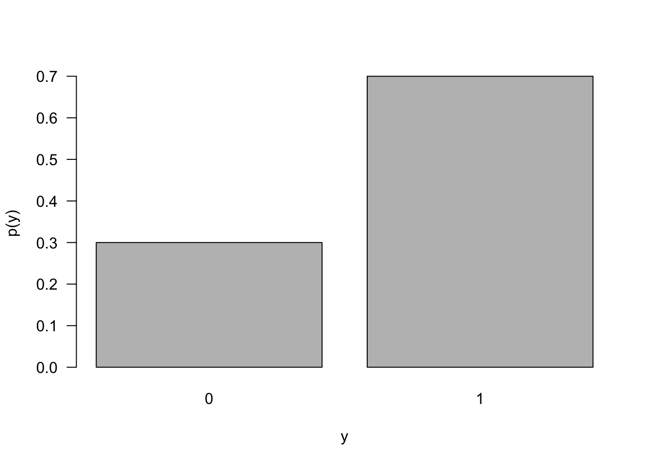
The mean and variance of the Bernoulli(\(\pi\)) random variable are \(\pi\) and \(\pi(1 - \pi)\), respectively—this was derived from first principles earlier. Notice that the variance is largest at \(\pi = 0.5\), when there is greatest uncertainty about which of the two events will occur.
Figure 59.1 displays the probability mass function of a Bernoulli random variable with event probability \(\pi = 0.7\).
Binomial, Binomial\((n,\pi)\)
Let \(Y_{1},\cdots,Y_{n}\) be independent binary experiments with the same event probability \(\pi\). Then the sum \(X = \sum_{i = 1}^{n}Y_{i}\) has a Binomial(\(n,\pi\)) distribution with p.m.f.
\[ \Pr(X = x) = \begin{pmatrix} n \\ x \end{pmatrix}\pi^{x}(1 - \pi)^{n - x},\ \ \ \ \ x = 0,1,\cdots,n \]
The mean and variance of the Binomial(\(n,\pi\)) variable can be found easily from its definition as a sum of independent Bernoulli(\(\pi\)) variables:
\[ \text{E}\lbrack X\rbrack = n\pi \qquad \text{Var}\lbrack X\rbrack = n\pi(1 - \pi) \]
The Bernoulli(\(\pi\)) distribution is the special case of the Binomial(\(1,\pi\)) distribution.
Geometric, Geometric\((\pi)\)
The Binomial(\(n,\pi\)) distribution is the number of events in a series of \(n\) Bernoulli(\(\pi\)) experiments. The Geometric(\(\pi\)) distribution also can be defined in terms of independent Bernoulli(\(\pi\)) experiments as the number of trials needed to obtain the first event. There is no theoretical upper bound for the support, as you might need infinitely many binary experiments to realize one event.
The p.m.f. of a Geometric(\(\pi\)) random variable, and its mean and variance, are given by
\[ p(x) = \pi(1 - \pi)^{x - 1}\ \ \ \ \ \ x = 1,2,\cdots \]
\[ \text{E}\lbrack X\rbrack = \frac{1}{\pi}\ \ \ \ \ \text{Var}\lbrack X\rbrack = \frac{1 - \pi}{\pi^{2}} \]
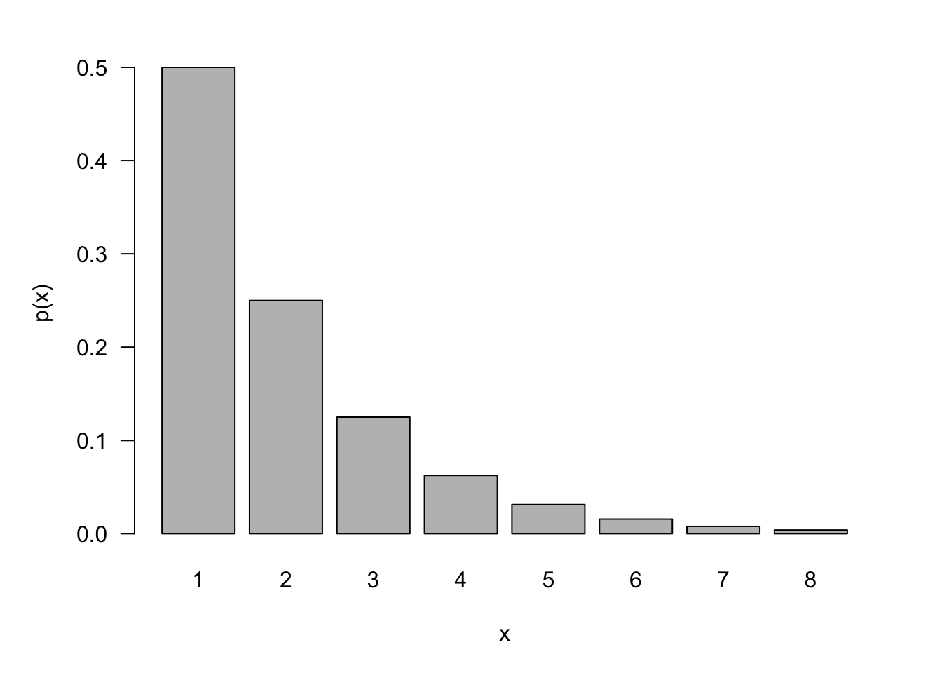
The following figure shows the p.m.f. of a Geometric(0.5) distribution. The probability to observe an event on the first try is 1/2, on the second try is 1/4, on the third try is 1/8, and so forth.
An interesting property of Geometric(\(\pi\)) random variables is their lack of memory:
\[ \Pr\left( X > s + t|X > t \right) = \Pr(X > s) \]
The probability that we have to try \(s\) more times to see the first event is independent of how many times we have tried before (\(t\)). To prove this note that \(\Pr(X > s)\) means the first event occurs after the \(s\)th try which implies that the first \(s\) tries were all non-events: \(\Pr{(X > s) = (1 - \pi)^{s}}\). The conditional probability in question becomes
\[\begin{align*} \Pr\left( X > s + t|X > t \right) &= \frac{\Pr{(X > s + t,\ X > t)}}{\Pr{(X > t)}} \\ &= \frac{\Pr{(X > s + t)}}{\Pr{(X > t)}} \\ &= \frac{(1 - \pi)^{s + t}}{(1 - \pi)^{t}} = (1 - \pi)^{s} \end{align*}\]
But the last expression is just \(\Pr{(X > s)}\).
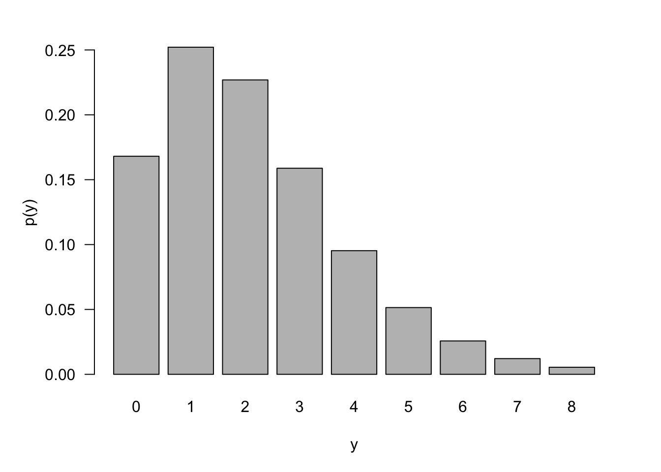
Please note that there is a second definition of the Geometric(\(\pi\)) distribution in terms of independent Bernoulli(\(\pi\)) experiments, namely as the number of non-events before the first event occurs. The p.m.f. of this random variable is
\[ p(y) = \pi(1 - \pi)^{y}\ \ \ \ \ y = 0,1,2,\cdots \]
With mean \(\text{E}\lbrack Y\rbrack = \frac{(1 - \pi)}{\pi}\) and variance \(\text{Var}\lbrack Y\rbrack = \frac{(1 - \pi)}{\pi}^{2}\).
Negative Binomial, NegBin\((k,\pi)\)
An extension of the Geometric(\(\pi\)) distribution is the Negative Binomial (NegBin(\(k,\pi\))) distribution. In a series of independent Bernoulli(\(\pi\)) trials, the number of experiments until the \(k\)th event is observed, is a NegBin(\(k,\pi\)) random variable.
A NegBin(\(k,\pi\)) random variable is thus the sum of \(k\) Geometric(\(\pi\)) random variables. The p.m.f., mean, and variance of \(X \sim \text{NegBin}(k,\pi)\) are
\[ p(x) = \begin{pmatrix} x - 1 \\ k - 1 \end{pmatrix}\pi^{k}(1 - \pi)^{x - k},\ \ \ \ \ x = k,k + 1,\cdots \]
\[\begin{align*} \text{E}\lbrack X\rbrack &= \frac{k}{\pi} \\ \text{Var}\lbrack X\rbrack &= \frac{k(1 - \pi)}{\pi^{2}} \end{align*}\]
The negative binomial distribution appears in many parameterizations. A popular form is in terms of the number of non-events before the \(k\)th event occurs. This changes the support of the random variable from \(x = k,k + 1,\cdots\) to \(y = 0,1,\cdots.\) The p.m.f,. mean, and variance of that random variable are
\[ p(y) = \begin{pmatrix} y + k - 1 \\ k - 1 \end{pmatrix}\pi^{k}(1 - \pi)^{y},\ \ \ \ y = 0,1,\cdots \]
\[\begin{align*} \text{E}\lbrack Y\rbrack &= \frac{k(1 - \pi)}{\pi} \\ \text{Var}\lbrack Y\rbrack &= \frac{k(1 - \pi)}{\pi^{2}} \end{align*}\]
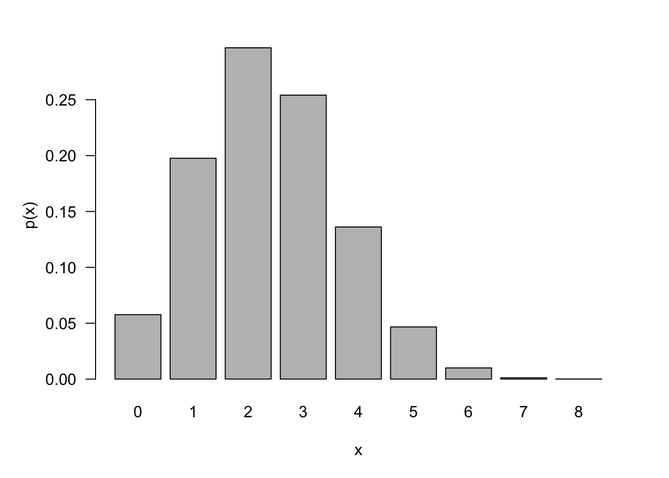
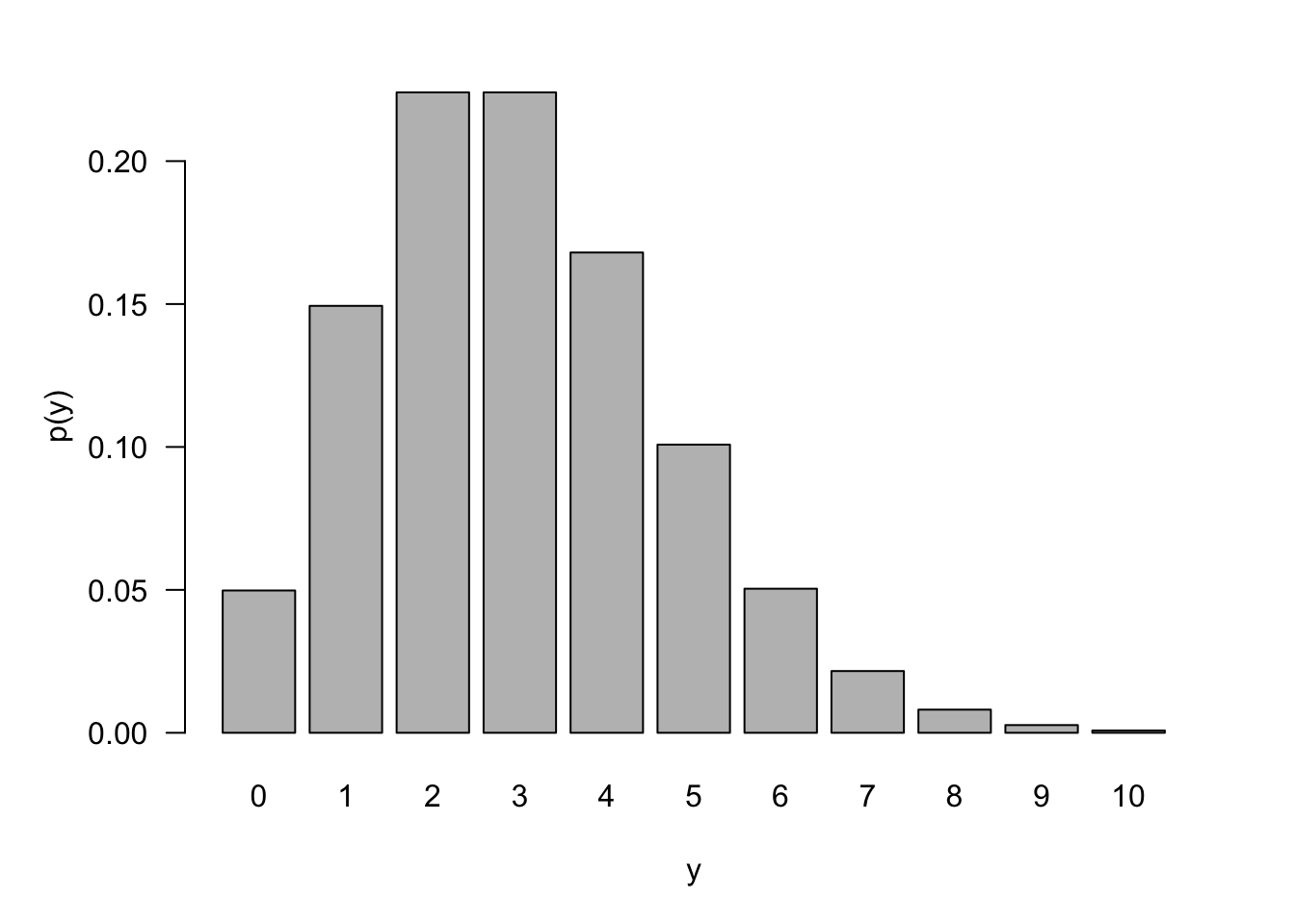
The p.m.f. for a NegBin(5,0.7) in this parameterization is shown in Figure 59.4.
An important application of the negative binomial distribution is in mixing models. These are models where the parameters of a distribution are assumed to be random variables rather than constants. This mechanism introduces additional variability into the system and is applied when the observed data appear more dispersed than a distribution permits. This condition is called overdispersion. For example, a binomial random variable has variance \(n\pi(1 - \pi)\); the variability is a function of the mean \(n\pi\). When the observed data suggest that this relationship between mean and variance does not hold—and typically the observed variability is greater than the nominal variance—one can treat \(n\) or \(\pi\) as a random variable. If you assume that \(n\) follows a Poisson distribution (see next), then the marginal distribution of the data is also Poisson. If you start with a Poisson distribution and assume that its parameter follows a Gamma distribution, the resulting marginal distribution of the data is negative binomial.
Poisson, Poisson\((\lambda)\)
The Poisson distribution is a common probability model for count variables that represent counts per unit, rather than counts that can be converted to proportions. For example, the number of chocolate chips on a cookie, the number of defective parts per day on an assembly line or the number of fish caught per day can be modeled as Poisson random variables.
The Poisson distribution as a model for random counts in time or space rests on three conditions:
- There are no multiple events at any point in time or space.
- The rate at which events occur is constant.
- Events in non-overlapping intervals occur independently of each other.
For the Poisson assumption to be met when modeling event counts over some unit, e.g. time, the rate at which events occur cannot depend on the occurrence of any events and events have to occur at a steady rate. For example, if the number of customer calls to a service center increases sharply after the release of a new software product, then the rate of events (calls) per day is not constant across days. This can still be modeled as a Poisson process where \(\lambda\) depends on other input variables such as the time since release of the new product. If one customer’s call makes it more likely that another customer calls into the service center, the Poisson assumption is not valid.
When modeling the emission of alpha particles from radioactive material, the assumption of a constant rate of emission is reasonable if the half-life of the material is much longer than the observation period.
The random variable \(Y\) has a Poisson(\(\lambda\)) distribution if its probability mass function is given by
\[ p(y) = \frac{e^{- \lambda\ }\lambda^{y}}{y!},\ \ \ \ y = 0,1,\cdots \]
The mean and variance of a Poisson(\(\lambda\)) variable are the same, \(\text{E}\lbrack Y\rbrack = \text{Var}\lbrack Y\rbrack = \lambda\). Although the random variable \(Y\) takes on only non-negative integer value, the parameter \(\lambda\) is a real number.
Example: Mean of the Poisson(\(\lambda\)) Distribution
We derive the mean here as an example how to manipulate probability mass functions. \[\begin{align*} \text{E}[Y] &= \sum_{y=0}^\infty y \ p(y) = \sum_{x=0}^\infty y \frac{\lambda^y e^-\lambda }{y!} \\ &= \sum_{y=1}^\infty \frac{\lambda^x e^-\lambda}{(y-1)!} \\ &= \lambda \sum_{y=0}^\infty \frac{\lambda^y e^-\lambda}{y!} \\ &= \lambda \end{align*}\]
After substituting the Poisson p.m.f., adjust the limit of summation because the first term equals 0 for \(y=0\). Then, pull out \(\lambda\) from the sum and you are left with the sum over the possible values of a Poisson random variable—which sums to 1.
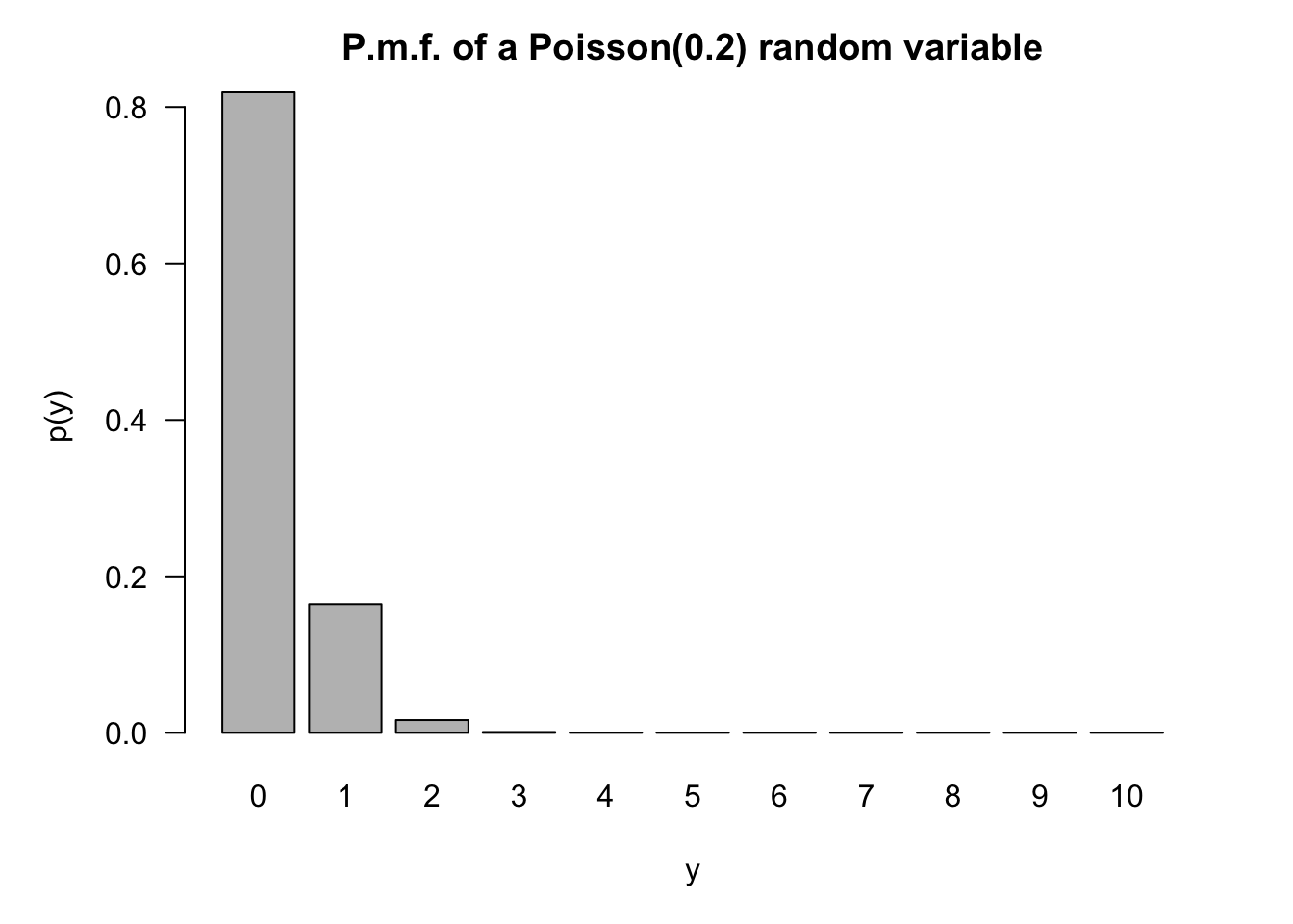
For larger values of \(\lambda\), the distribution shifts to the right and becomes more symmetric (Figure 59.5). For small values of \(\lambda\), the mass function is very asymmetric and concentrated at small values of \(Y\) (Figure 59.6).
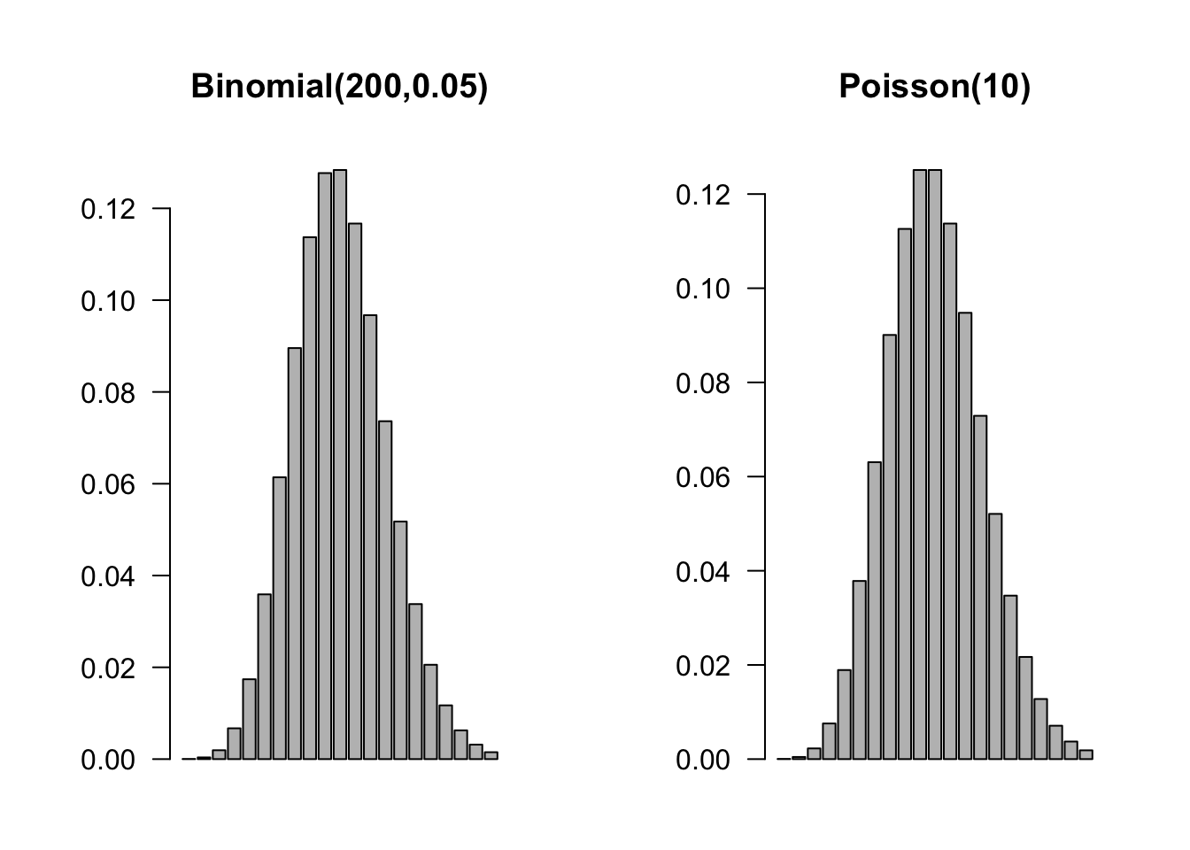
This is the basis for the Poisson approximation to Binomial probabilities. In a Binomial(\(n,\pi\)) process, if \(n \rightarrow \infty\) and \(\pi\) shrinks so that \(n\pi\) converges to a constant \(\lambda\), then the Binomial(\(n,\pi\)) process can be approximated as a Poisson(\(\lambda\)) process. Figure 59.7 compares a Binomial(200,0.05) mass function to the p.m.f. of the Poisson(10). At least visually, the histograms are almost indistinguishable.
For example, the probability that three sixes turn up when three dice are rolled is \(\frac{1}{216} = 0.00463\). If the three dice are rolled 200 times, what is the probability that at least one triple six shows up? If \(Y\) is the number of triple sixes out of 200, then the binomial probability is calculated as
\[ 1 - \begin{pmatrix} 200 \\ 0 \end{pmatrix}\left( \frac{1}{216} \right)^{0}\left( \frac{215}{216} \right)^{200} = 0.6046\]
and the Poisson approximation is
\[ 1 - \frac{\left( \frac{200}{216} \right)^{0}}{0!}\exp\left\{ - \frac{200}{216} \right\} = 0.6038 \]
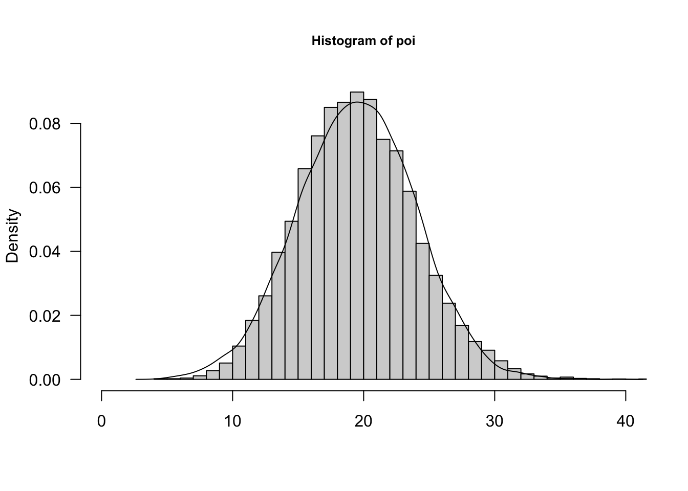
As \(\lambda \rightarrow \infty\), the Poisson p.m.f. approaches the shape of a Gaussian (normal) distribution. Some folks recommend the Gaussian approximation for the Poisson for \(\lambda > 100\) or even \(\lambda > 1000\). The approximation is sometimes made for smaller values of the Poisson parameter. Figure 59.8 shows the empirical histogram and density for 10,000 random draws from a Poisson(20) distribution and a Gaussian distribution with the same mean and variance as the Poisson. The approximation works quite well.
Because the events being counted occur independently of each other, a Poisson distribution is divisible. You can think of a Poisson(\(\lambda = 5\)) variable as the sum of five Poisson(1) variables. The result of one variable producing on average 5 events per time units or five variables each producing on average one event per unit is the same. More generally, if \(Y_{1},\cdots,Y_{n}\) are independent random variables with respective Poisson(\(\lambda_{i}\)) distributions, then their sum \(\sum_{i=1}^{n}Y_{i}\) follows a Poisson distribution with mean \(\lambda = \sum_{i=1}^{n}\lambda_{i}\).
59.5 Continuous (Univariate) Distributions
For continuous random variables, the probability that the variable takes on any particular value is zero. To make meaningful probability statements we consider integration of the probability density function (p.d.f.) over sets, for example, intervals:
\[\Pr{(a \leq X \leq b)} = \int_{a}^{b}{f(x)dx}\]
The density function satisfies \(\int_{- \infty}^{\infty}{f(x)dx} = 1\) and can be obtained by differentiating the c.d.f \(F(x) = \Pr{(X \leq x)}\); \(f(x) = \frac{dF(x)}{dx}\).
Uniform, U\((a,b)\)
If a random variable has a continuous uniform distribution on the interval \(\lbrack a,b\rbrack\), denoted \(Y \sim U(a,b)\), its p.d.f. is given by
\[ f(x) = \left\{ \begin{matrix} \frac{1}{(b - a)} & a \leq x \leq b \\ 0 & \text{otherwise} \end{matrix} \right.\ \]
The mean and variance of a \(U(a,b)\) random variable are
\[ \text{E}\lbrack Y\rbrack = \frac{a + b}{2}\ \ \ \ \ \ \text{Var}\lbrack Y\rbrack = \frac{(b - a)^{2}}{12} \]
Exponential, Expo\((\lambda)\)
The exponential distribution is a useful probability model for modeling continuous lifetimes. It is related to Poisson processes. If events occur continuously and independently at a constant rate \(\lambda\), the number of events is a Poisson random variable. The time between the events is an exponential random variable, denoted \(Y \sim\) Expo(\(\lambda\)).
\[\begin{align*} p(y) &= \lambda e^{- \lambda y},\ \ \ \ y \geq 0 \\ F(y) &= 1 - e^{- \lambda y},\ \ \ y \geq 0 \\ \text{E}\lbrack Y\rbrack &= \frac{1}{\lambda} \\ \text{Var}\lbrack Y\rbrack &= \frac{1}{\lambda^{2}} \end{align*}\]
Like the discrete Geometric(\(\pi\)) distribution, the Expo(\(\lambda\)) distribution is forgetful,
\[ \Pr{(Y > s + t|Y > t)} = \Pr{(Y > s)} \]
and it turns out that no other continuous function has this memoryless property. This property is easily proven using \(\Pr(Y > y) = 1 - F(y) = e^{- \lambda y}\):
\[\begin{align*} \Pr\left( Y > t + s \middle| Y > t \right) &= \frac{\Pr{(Y > t + s,Y > t)}}{\Pr{(Y > t)}}\\ &= \frac{Pr(Y > t + s)}{Pr(Y > t)} \\ &= \frac{e^{- \lambda(t + s)}}{e^{- \lambda t}} = e^{- \lambda s} \end{align*}\]
The memoryless property of the exponential distribution makes it not a good model for human lifetimes. The probability that a 20-year-old will live another 10 years is not the same as the probability that a 75-year-old will live another 10 years. The exponential distribution implies that this would be the case and is not an appropriate model. However, when modeling earthquakes, it might be reasonable to stipulate that the probability of an earthquake in the next ten years is the same, regardless of when the last earthquake occurred—the exponential distribution would then be reasonable.
You don’t have to worry about whether other distributions have this memoryless property in applications where lack of memory would not be appropriate. The exponential distribution is defined by this property, it is the only continuous distribution with lack of memory.
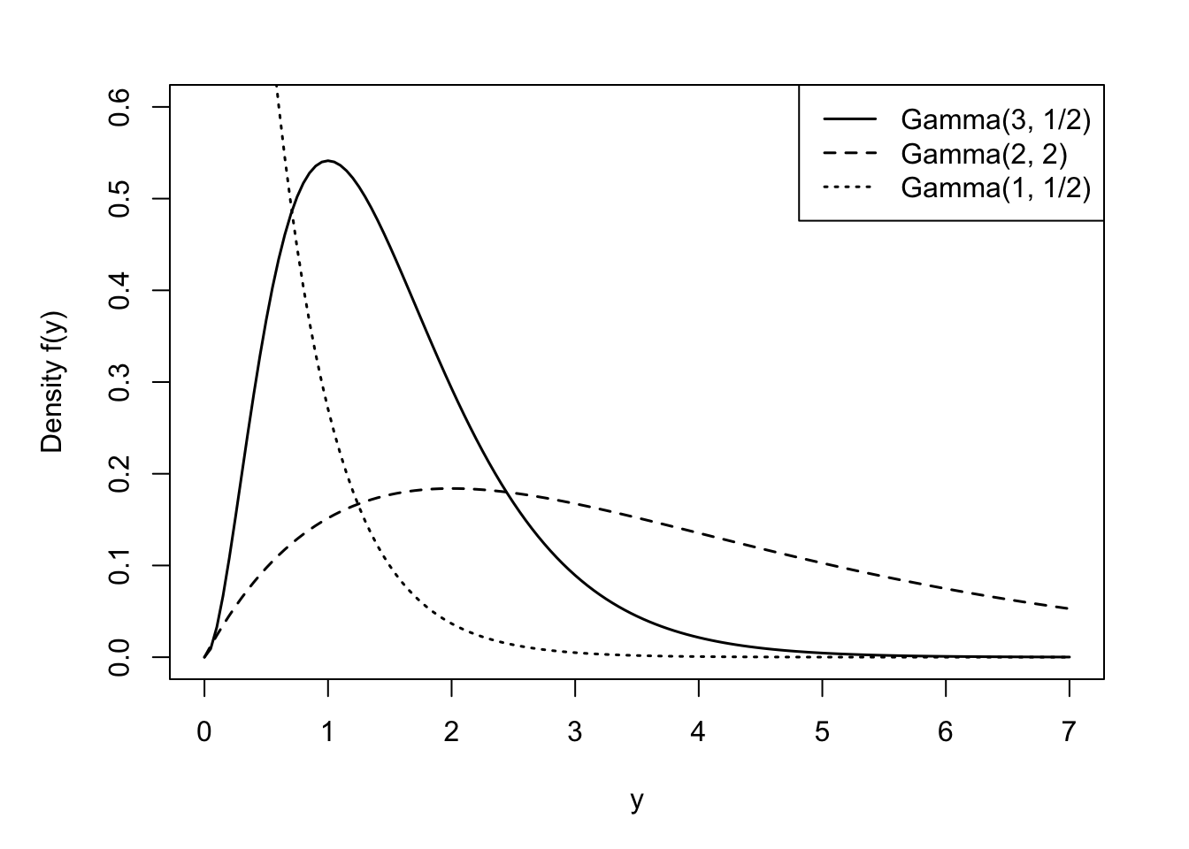
Gamma, Gamma\((\alpha,\beta)\)
The Expo(\(\lambda\)) distribution is a special case of a broader family of distributions, the Gamma(\(\alpha,\beta\)) distribution. A random variable \(Y\) is said to have a Gamma(\(\alpha,\beta\)) distribution if its density function is
\[ f(y) = \frac{1}{\beta^{\alpha}\Gamma(\alpha)}y^{\alpha - 1}e^{- y/\beta}, \qquad y \geq 0,\ \alpha,\beta > 0 \tag{59.1}\]
The mean and variance of a Gamma(\(\alpha,\beta\)) random variable are given by
\[\begin{align*} \text{E}\lbrack Y\rbrack &= \alpha\beta \\ \text{Var}\lbrack Y\rbrack &= \alpha\beta^{2} \end{align*}\]
\(\alpha\) is called the shape parameter of the distribution and \(\beta\) is called the scale parameter. Varying \(\alpha\) affects the shape and varying \(\beta\) affects the units of measurement.
The term \(\Gamma(\alpha)\) in the denominator of the density function is called the Gamma function,
\[ \Gamma(\alpha) = \int_{0}^{\infty}{y^{\alpha - 1}e^{- y}}dy \]
Tip
Fun fact: if \(\alpha\) is an integer, \(\Gamma(\alpha) = (\alpha - 1)!\)
The exponential random variable introduced earlier is a special case of the Gamma family, the Expo(\(1/\beta\)) is the same as the Gamma(1,\(\beta\)). Gamma-distributed random variables occur in applications of waiting times. Suppose that cars arrive at an intersection at a rate of one every two minutes. The time you have to wait until the 5th car arrives at the intersection is a Gamma(\(\alpha=5,\beta=2\)) random variable. If lightbulbs last 5 years on average are replaced when they fail, the time a box of six lasts is a Gamma(\(\alpha=6, \beta=5\)) random variable (Cunningham 2024).
Another special case of the gamma-type random variables is the chi-square random variable. A random variable \(Y\) is said to have a chi-squared distribution with \(\nu\) degrees of freedom, denoted \(\chi_{\nu}^{2}\), if \(Y\) is a Gamma(\(\frac{\nu}{2},2\)) random variable. More on \(\chi^{2}\) random variables below after we introduced sampling from a Gaussian distribution.
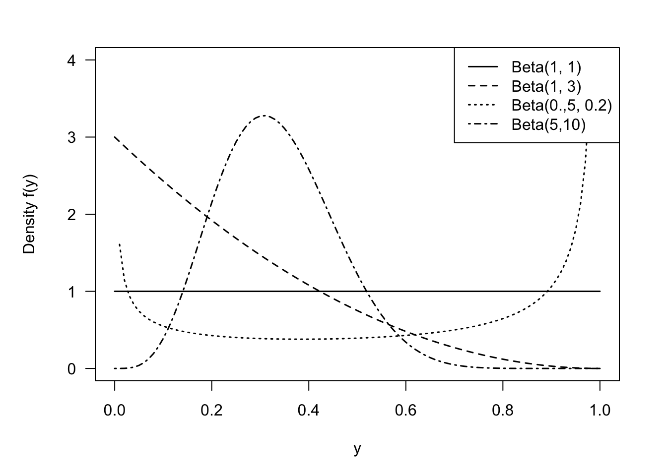
Beta, Beta\((\alpha,\beta)\)
A random variable has a Beta distribution with parameters \(\alpha\) and \(\beta\), denoted \(Y \sim \text{Beta}(\alpha,\beta)\), if its density function is given by \[ f(y) = \frac{\Gamma(\alpha+\beta)}{\Gamma(\alpha)\Gamma(\beta)}\, y^{\alpha-1}\,(1-y)^{\beta-1}\quad 0 < y < 1 \] The family of beta distributions takes on varied shapes as seen in Figure 59.10.
The ratio of Gamma functions is known as the Beta function and the density can also be written as \(f(y) = y^{\alpha-1}(1-y)^{(\beta-1)} / B(\alpha,\beta)\) where \(B(\alpha,\beta) = \Gamma(\alpha)\Gamma(\beta)/\Gamma(\alpha+\beta)\).
The mean of a \(\text{Beta}(\alpha,\beta])\) random variable is \[ \text{E}[Y] = \frac{\alpha}{\alpha+\beta} \] and the variance is \[ \text{Var}[Y] = \frac{\alpha\beta}{(\alpha+\beta)^2 (\alpha+\beta+1)} = \text{E}[Y]\frac{\beta}{(\alpha+\beta)(\alpha+\beta+1)} \]
The support of a Beta random variable is continuous on [0,1], which makes it an attractive candidate for modeling proportions, for example, the proportion of time a vehicle is in maintenance or the proportion of disposable income spent on rent. Cunningham (2024) gives the following examples of Beta distributions:
- Five numbers are chosen at random from the interval (0,1) and arranged in order. The middle number has a Beta(3,3) distribution.
- The probability that an apple will be unblemished has a Beta(8,0.5) distribution.
- Relative humidity for Auckland, New Zealand for the first six months of 2022 has an approximate Beta(5.93, 1.78) distribution.
The Beta distribution can also be used for random variables that are defined on a different scale, \(a < Y < b\) by transforming to the [0,1] scale: \(Y^* = (Y-a)/(b-a)\).
Here are some interesting properties and relationships for Beta random variables:
The \(\text{Beta}(1,1)\) is a continuous uniform random variable on [0,1].
If \(Y \sim \text{Beta}(\alpha,\beta)\), then \(1 - Y \sim \text{Beta}(\beta,\alpha)\).
The relationship between Gamma and Beta functions hints at a relationship between Gamma and Beta random variables. Indeed, there is one. If \(X \sim \text{Gamma}(\alpha_1,\beta)\) and \(Y \sim \text{Gamma}(\alpha_2,\beta)\), and \(X\) and \(Y\) are independent, then the ratio \(X/(X+Y)\) follows a Beta\((\alpha_1,\alpha_2)\) distribution:
\[ \frac{X}{X+Y} \sim \text{Beta}(\alpha_1,\alpha_2) \]
- If \(X\) is an Expo(\(\lambda\)) random variable then \(e^{−X} \sim \text{Beta}(\lambda,1)\).
Since \(Y\) is continuous, we can define the support of the Beta random variable as \(0 \le y \le 1\) or as \(0 < y < 1\). The probability that the continuous random variable takes on exactly the value 0 or 1 is zero. However, in practice you can observe proportions at the extreme of the support; the proportion of income spent on rent by a homeowner is zero.
Gaussian (Normal), G\((\mu,\sigma^2)\)
The Gaussian (or Normal) distribution is arguably the most important continuous distribution in all of probability and statistics. A random variable \(Y\) has a Gaussian distribution with mean \(\mu\) and variance \(\sigma^{2}\), if its density function is
\[ f(y) = \frac{1}{\sqrt{2\pi\sigma^{2}}}\exp\left\{ - \frac{1}{2\sigma^{2}}(y - \mu)^{2} \right\},\quad -\infty < y < \infty \]
The notation \(Y \sim G\left( \mu,\sigma^{2} \right)\) or \(Y \sim N\left( \mu,\sigma^{2} \right)\) is common.
The Gaussian distribution has the famous bell shape, symmetric about the mean \(\mu\).
A special version is the standard Gaussian (standard normal) distribution \(Z \sim G(0,1)\) with density
\[ f(z) = \frac{1}{\sqrt{2\pi}}\exp\left\{ - \frac{1}{2}y^{2} \right\} \]
The standard Gaussian is also referred to as the unit normal distribution.
Gaussian random variables have some interesting properties. For example, linear combinations of Gaussian random variables are Gaussian distributed. If \(Y\sim G\left( \mu,\sigma^{2} \right)\), then \(X = aY + b\) has distribution \(G(a\mu + b,a^{2}\sigma^{2})\). As an example, if \(Y\sim G\left( \mu,\sigma^{2} \right)\), then
\[ Z = \frac{Y - \mu}{\sigma} \]
has a standard Gaussian distribution. You can express probabilities about \(Y\) in terms of probabilities about \(Z\):
\[ \Pr{(X \leq x)} = \Pr\left( Z \leq \frac{x - \mu}{\sigma} \right) \]
Because linear functions of Gaussian random variables are Gaussian random variables, it is easy to establish the distribution of the sample mean \(\overline{Y} = \frac{1}{n}\sum_{i}^{}Y_{i}\) in a random sample from a \(G(\mu,\sigma^{2})\) distribution. First, if we take a random sample from any distribution with mean \(\mu\) and variance \(\sigma^{2}\), then the sample mean \(\overline{Y}\) has mean and variance
\[\begin{align*} \text{E}\left\lbrack \overline{Y} \right\rbrack &= \mu \\ \text{Var}\left\lbrack \overline{Y} \right\rbrack &= \frac{\sigma^{2}}{n} \end{align*}\]
This follows from the linearity of the expectation operator and the independence of the observations in the random sample. If, in addition, the \(Y_{i} \sim G\left( \mu,\sigma^{2} \right)\), then
\[ \overline{Y} \sim G\left( \mu,\frac{\sigma^{2}}{n} \right) \]
The sample mean of a random sample from a Gaussian distribution also has a Gaussian distribution. Do we know anything about the distribution of \(\overline{Y}\) if we randomly sample a non-Gaussian distribution? Yes, we do. That is the domain of the central limit theorem.
Central Limit Theorem
Let \(Y_{1},\cdots,Y_{n}\) be independent and identically distributed random variables with mean \(\mu\) and variance \(\sigma^{2} < \infty.\) The distribution of
\[\frac{\overline{Y} - \mu}{\sigma/\sqrt{n}}\]
converges to that of a standard Gaussian random variable as \(n \rightarrow \infty\).
These amazing properties contribute to the Gaussian distribution being the most important probability distribution. Most continuous attributes actually do not behave like Gaussian random variables at all, they often have a restricted range or are skewed or have heavier tails than a Gaussian random variable. There is really nothing normal about this distribution, which is one reason why we prefer the name Gaussian over Normal distribution.
What is normal?
We avoid the use of the term normal to describe the Gaussian distribution for another reason: the connection of the concept of normality and this distribution to eugenics. The Belgian astronomer, statistician and mathematician Adolphe Quetelet (1796–1847) introduced the generalized notion of the normal. He studied the distribution of physical attributes and determined that the normal, the most representative, value of an attribute is its average. Discrepancies above and below the average were considered “errors”. Early applications of the Gaussian distribution were in the study of measurement errors. C.F. Gauss used the distribution to represent errors in the measurement of celestial bodies.
Prior to Quetelet, the view of “norm” and “normality” was associated with carpentry. The carpenter square is also called the norm, and in normal construction everything is at right angles. With Quetelet, the middle of the distribution, the center, became the “new normal.” There is nothing objectionable so far.
This view did not sit well with Francis Galton, however, who introduced the term eugenics. Galton replaced the term “error” with standard deviation and considered variability within a human population as potential for racial progress (Grue and Heiberg 2006). The bell shape of the normal distribution was not used to focus our attention on the average, as Quetelet did. Galton introduced quartiles to categorize the area under the distribution into sections of greater and lesser genetic worth. That is not normal!
59.6 Probability and Likelihood
The terms probability and likelihood are often used interchangeably, but they do mean different things. TLDR: probabilities are attached to outcomes (data), likelihoods are attached to hypotheses (parameters).
Suppose random variable \(X\) has a Binomial(10, 0.7) distribution. We know the parameters of the distribution, \(n=10\), \(\pi=0.7\), and ask questions about the possible outcomes under this model. The support of \(X\) is \(\{0,1,\cdots,10\}\) and the probabilities sum to one over the support: \[ \sum_{i=0}^{10} \Pr(X=i | X\sim \text{ Binomial}(10, 0.7)) = 1 \]
The likelihood is sometimes called a reverse probability because it turns the question around: given that we have seen a particular outcome, what is the support of a certain hypothesis? The outcome is the data we observe, the hypothesis is about values of the model parameters. So, if we observe 6 events out of 10 in the Binomial model, we can ask how likely this outcome is if the event probability is 0.5. Or if it is 0.1, or 0.6, or 0.8.
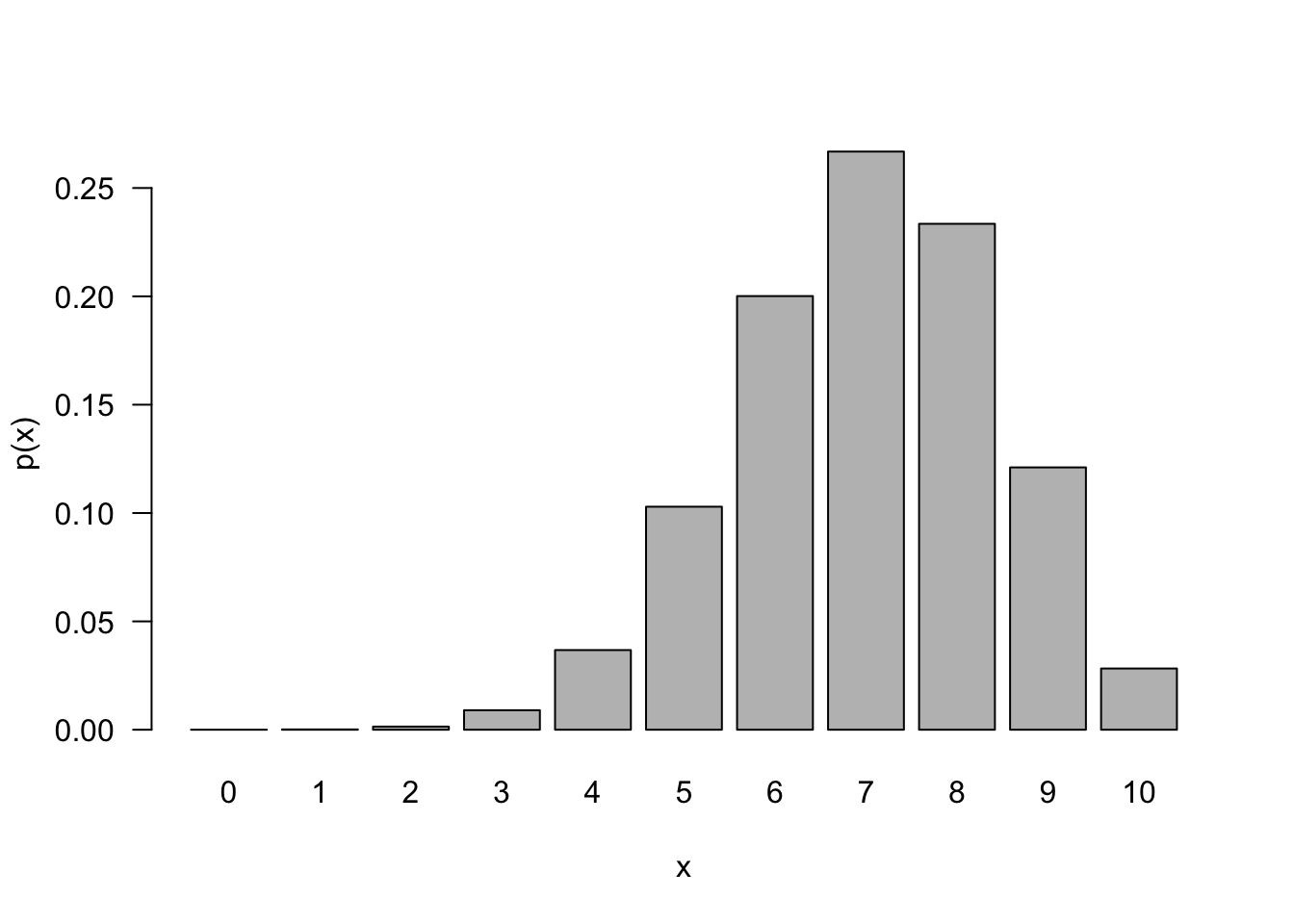
The likelihood function makes statements about the parameters given the data. The probability density or mass functions tells us about the occurrence of data given the parameters. Figure 59.12 shows the probabilities \(\Pr(X=0)\) through \(\Pr(X=10)\) if \(X \sim \text{ Binomial}(10, 0.7)\).
Probabilities of mutually exclusive outcomes sum (or integrate) to meaningful quantities. Likelihoods, on the other hand do not have any meaningful scale. What matters with likelihoods is the relative magnitude of one likelihood versus another. For example, the likelihood that \(\pi = 0.5\) if we observe 6 out of 10 events can be compared against the likelihood that \(\pi = 0.6\). This likelihood ratio gives us an idea how much more plausible it is that \(\pi = 0.6\) than \(\pi = 0.5\). Maximum likelihood estimation is the principle to choose as estimates of unknown parameters those values that have the largest likelihood, these are the most plausible values given the data that was observed.
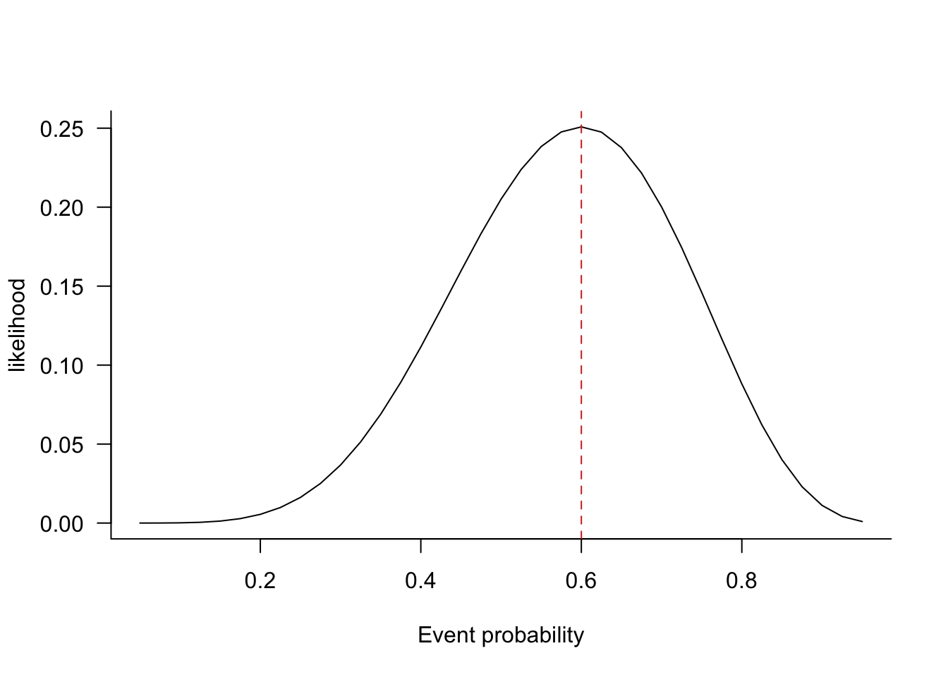
Figure 59.13 shows the likelihood function for a binomial experiment with 6 out of 10 successes. The likelihood for a particular parameter value, say \(\pi_0\), is obtained by calculating the probability \(\Pr(X=6 | \pi=\pi_0)\). Each point of the likelihood function corresponds to a different parameter value, hence the function does not integrate to anything meaningful. The most plausible value for the parameter, the maximum likelihood estimate, is \(\widehat{\pi} = 6/10=0.6\); where the likelihood function reaches a maximum.
59.7 Moment Generating Functions
The moment generating function (MGF) of a random variable \(X\) is \[ M_x(t) = \text{E}\left[e^{tX}\right] \]
By first principles, if \(X\) is discrete, \(X \in \{x_1,x_2,\cdots\}\), \[ M_x(t) = \sum_{i=1}^\infty e^{tx_i} \ p(x_i) \] and if \(X\) is continuous, \[ M_x(t) = \int_{-\infty}^\infty e^{tx}\ f(x) \ d(x) \]
The name comes from the fact that the function can be used to—wait for it—generate the moments of \(X\). To see how this works, consider the Taylor series of \(e^{tX}\): \[
e^{tX} = 1 + \frac{tX}{1!} + \frac{t^2X^2}{2!} + \frac{t^3X^3}{3!} + \cdots + \frac{t^nX^n}{n!} + \cdots
\] Take the expectation of the series and you get \[
\text{E}[e^{tX}] = 1 + \frac{t\text{E}[X]}{1!} + \frac{t^2\text{E}[X^2]}{2!} + \frac{t^3\text{E}[X^3]}{3!} + \cdots + \frac{t^n\text{E}[X^n]}{n!} + \cdots
\] Note that we consider the MGF as a function of \(t\). The first derivative of the MGF with respect to \(t\) is \[
\frac{\partial \text{E}[e^{tX}]}{\partial t} = \frac{\text{E}[X]}{1!} + 2\frac{t\text{E}[X^2]}{2!} + 3\frac{t^2\text{E}[X^3]}{3!} + \cdots + n\frac{t^{n-1}\text{E}[X^n]}{n!} + \cdots
\] Evaluating this derivative at \(t=0\) yields \(\text{E}[X]\).
Similarly, the second derivative with respect to \(t\) is \[
\frac{\partial^2 \text{E}[e^{tX}]}{\partial t^2} = 2\frac{\text{E}[X^2]}{2!} + 6\frac{t\text{E}[X^3]}{3!} + \cdots + n(n-1)\frac{t^{n-2}\text{E}[X^n]}{n!} + \cdots
\] Evaluating this derivative at \(t=0\) yields \(\text{E}[X^2]\).
More generally, the \(r\)th derivative of the MGF with respect to \(t\) is \[\begin{align*} \frac{\partial^r M_x(t)}{\partial t^r} &= \frac{\partial^r}{\partial t^r} \int_{-\infty}^\infty e^{tx}\ f(x) \ dx \\ &= \int_{-\infty}^\infty x^r e^{tx}\ f(x) \ dx \end{align*}\]
If you evaluate this integral at \(t=0\), you get the \(r\)th moment of \(X\): \[ \frac{\partial^r M_x(t)}{\partial t^r}_{\lvert{t=0}} = \int_{-\infty}^\infty x^r f(x) \ dx = \text{E}[X^r] \]
Table 59.2 lists the MGF of some well-known distributions. Note that a MGF does not necessarily exist.
| Distribution | \(M_x(t)\) |
|---|---|
| Uniform (continuous) | \(\frac{e^{tb} - e^{ta}}{t(b-a)}\) |
| Uniform (discrete) | \(\frac{e^{at} - e^{(b+1)t}}{(b-a+1)(1-e^t)}\) |
| Gaussian | \(\exp\left\{t\mu + \frac12 t^2\sigma^2 \right\}\) |
| Gamma | \(\left(1-\beta t\right)^{-\alpha}\) |
| Chi-square | \((1-2t)^{\nu/2}, \ t < \frac12\) |
| T | does not exist |
| F | does not exist |
| Bernoulli | \(1-\pi+\pi e^t\) |
| Binomial | \(\left(1-\pi+\pi e^t\right)^n\) |
| Geometric \(\pi(1-\pi)^x\) | \(\frac{\pi}{1-(1-\pi)e^t}\) |
| Poisson | \(\exp\left\{\lambda(e^t-1)\right\}\) |
Here are examples of finding mean and variance of two distributions from the moment generating function.
Example: Mean and Variance of Poisson(\(\lambda\))
The probability mass function of the Poisson(\(\lambda\)) distribution is \[ p(x) = \frac{e^{-\lambda}\lambda^x}{x!} \quad x=0,1,2,\cdots \] It can be shown that the moment generating function is \[ M(x)(t) = \exp\left\{\lambda(e^t-1)\right\} \] To find the first two moments, \(\text{E}[X]\) and \(\text{E}[X^2]\): \[ \text{E}[X] = \frac{\partial M_X(t)}{\partial t}_{\lvert{t=0}} = e^{-\lambda}\lambda e^t \exp\{\lambda e^t\}_{\lvert{t=0}} = \lambda \] \[ \text{E}[X^2] = \frac{\partial^2 M_X(t)}{\partial t^2}_{\lvert{t=0}} = e^{-\lambda}\lambda e^t \exp\{\lambda e^t\}_{\lvert{t=0}} + e^{-\lambda} \lambda^2 e^{2t}\exp\{\lambda e^t\}_{\lvert{t=0}} = \lambda + \lambda^2 \] The variance of \(X\) follows as \(\text{Var}[X] = \text{E}[X^2] - \text{E}[X]^2 = \lambda + \lambda^2 - \lambda^2 = \lambda\).
Example: Mean and Variance of Gamma(\(\alpha,\beta\))
The density function of a Gamma(\(\alpha,\beta\))-distributed random variable \(X\) is \[ f(x) = \frac{1}{\beta^{\alpha}\Gamma(\alpha)}x^{\alpha - 1}e^{- x/\beta},\ \ \ \ \ x \geq 0,\ \alpha,\beta > 0 \] and its moment generating function is \[ M_x(t) = \left(1-\beta t\right)^{-\alpha} \] The first and second derivatives of \(M_x(t)\) with respect to \(t\) are \[\begin{align*} \frac{\partial M_x(t)}{\partial t} &= \alpha\beta \left(1-\beta t\right)^{-\alpha - 1}\\ \frac{\partial^2 M_x(t)}{\partial t^2} &= \alpha(\alpha+1)\beta^2\left(1-\beta t\right)^{-\alpha - 2} \end{align*}\]
Evaluating the derivatives at \(t=0\) you get \[\begin{align*} \text{E}[X] &= \frac{\partial M_x(t)}{\partial t}_{\lvert{t=0}} = \alpha\beta \\ \text{E}[X^2] &= \frac{\partial^2 M_x(t)}{\partial t^2}_{\lvert{t=0}} = \alpha(\alpha+1)\beta^2 \\ \end{align*}\]
The variance of \(X\) follows easily: \[ \text{Var}[X] = \text{E}[X^2] - \text{E}[X]^2 = \alpha(\alpha+1)\beta^2 - \alpha^2\beta^2 = \alpha\beta^2 \]
Moment generating functions are also useful to find the distribution of a random variable. This is due to the uniqueness theorem: if two variables \(X\) and \(Y\) have the same MGF for all values for \(t\), then they have the same distribution. So, if you know the distribution of \(X\) and want to find the distribution of \(Y\), compare \(M_y(t)\) and \(M_x(t)\).
59.8 Functions of Random Variables
If random variable \(X\) has p.d.f. \(f(x)\), how can we find the density function of a transformation \(Y=g(X)\) of \(X\)? Three methods are commonly employed, relying on distribution functions, transformations, and moment generating functions.
Method of Distribution Functions
This methods finds the cumulative distribution function by integrating the density of \(X\) over the region for which \(Y = g(X) \le y\). The density of \(Y\) is then found by differentiation.
We learned previously about a famous property of Gaussian random variables: linear combinations of Gaussian r.v.s are also Gaussian distributed. We can prove that by deriving the distribution of \(Y = aX + b\) (\(a > 0\)) from the distribution of \(X \sim G(\mu,\sigma^2)\). Using \(F_y\), \(f_y\) and \(F_x\), \(f_x\) to denote c.d.f. and p.d.f. for \(Y\) and \(X\), respectively, we can express \(F_y\) in terms of \(F_x\):
\[ \begin{align*} F_y(y) &= \Pr(Y \leq y) = \Pr(aX+b \leq y) \\ &= \Pr\left(X \leq \frac{y-b}{a}\right) \\ &= F_x\left(\frac{y-b}{a}\right) \end{align*} \] To find the density function \(f_y\) in terms of the density of \(X\), take derivatives with respect to \(y\) of the right hand side:
\[ f_y(y) = \frac{d\,F_y(y)}{d \, y} = \frac{d}{d\,y}F_x\left(\frac{y-b}{a}\right) = \frac{1}{a}f_x\left(\frac{y-b}{a}\right) \tag{59.2}\]
So far, the Gaussian property of \(X\) has not come into play; Equation 59.2 applies to all distribution functions, provided that \(F_x\) can be differentiated. For the specific case where \(X \sim G(\mu,\sigma^2)\), the p.d.f. of \(X\) is \[ f(x) = \frac{1}{\sqrt{2\pi}\sigma} \exp\left\{ -\frac{1}{2} \left( \frac{x-\mu}{\sigma}\right)^2\right\} \] and \(\frac{1}{a} f_x((y-b)/a))\) is \[ \begin{align*} f_y(y) &= \frac{1}{a\sqrt{2\pi}\sigma} \exp\left\{-\frac{1}{2} \left(\frac{(y-b)/a - \mu}{\sigma}\right)^2 \right\} \\ &= \frac{1}{\sqrt{2\pi}a\sigma} \exp\left\{-\frac{1}{2} \left(\frac{y-(a\mu + b)}{a\sigma}\right)^2 \right\} \end{align*} \] This is the density of a \(G(a\mu + b,a^2\sigma^2)\) random variable.
Example: Density of \(Z^2\) when \(Z \sim G(0,1)\).
To find the distribution of \(X=Z^2\), where \(Z\) is a standard Gaussian, using the method of distribution functions, let \(\Phi(x)\) denote the c.d.f. and \(\phi(x)\) the p.d.f. of the \(G(0,1)\). \[\begin{align*} F_X(x) &= \Pr(X \le x) = \Pr(-\sqrt{x} \le X \le \sqrt{x}) \\ &= \Phi(\sqrt{x}) - \Phi(-\sqrt{x}) \end{align*}\]
Now differentiate with respect to \(x\) to find the density. Applying the chain rule of calculus gives \[ f_X(x) = \frac12 x^{-1/2}\phi(\sqrt{x}) + \frac12x^{-1/2}\phi(-\sqrt{x}) = x^{-1/2}\phi(\sqrt{x}) \] The symmetry of the Gaussian distribution was used to collapse the two terms into one. Plugging in the p.d.f of the standard Gaussian, this evaluates to \[ f_X(x) = \frac{x^{-1/2}}{\sqrt{2\pi}} \ e^{-x/2}, \quad x \ge 0 \]
This is the density of a chi-square distribution with one degree of freedom, a special case of the Gamma density.
This technique for deriving the density of a transformation of a random variable directly is useful to establish other famous relationships between random variables. For example, if \(X \sim G(0,1)\), what is the distribution of \(Y = X^2\)? To solve this we start with a probability statement about \(Y\) and translate it into a probability statement about \(X\). (We use the notation \(\Phi(x)\) and \(\phi(x)\) to denote the standard Gaussian c.d.f and p.d.f, respectively).
\[ \begin{align*} F_y(y) = \Pr(Y \leq y) &= \Pr(-\sqrt{y} \leq X \leq \sqrt{y}) \\ &= \Phi(\sqrt{y}) - \Phi(-\sqrt{y}) \end{align*} \] Taking derivatives with respect to \(y\) yields the density of \(Y\) in terms of the density of \(X\): \[ \begin{align*} f_y(y) &= \frac{1}{2}y^{-1/2}\phi\left(\sqrt{y}\right) + \frac{1}{2}y^{-1/2}\phi\left(-\sqrt{y}\right)\\ &= y^{-1/2}\phi\left(\sqrt{y}\right) \end{align*} \]
Plugging into the formula for the standard Gaussian density, the density of \(Y\) becomes \[ f_y(y) = \frac{y^{-1/2}}{\sqrt{2\pi}} \, \exp\{-y/2\} \] Compare this expression to Equation 59.1, it turns out that \(Y\) has a Gamma density with parameters \(\alpha = 1/2\), \(\beta=2\). This special case is also known as a chi-square distribution with one degree of freedom. More on chi-square distributions in Section 60.3.
Method of Transformations
This method of finding the distribution of \(Y = g(X)\), if the distribution of \(X\) is known, is a variation of the method of distribution functions. We require that \(g(X)\) is an increasing or decreasing function of \(X\), in the sense that if
\(x_1 < x_2\) then \(g(x_1) < g(x_2)\) and if \(x_1 > x_2\) then \(g(x_1) > g(x_2)\). In this situation we can find the inverse function \(X = g^{-1}(Y)\). After calculating the derivative \(dx/dy\), the density of \(Y\) is found as \[
f_y(y) = f_x(y) \left | \frac{dx}{dy} \right |
\tag{59.3}\]
An example will make the method of transformation clear.
Example: Method of Transformation
Suppose that \(X\) has density function \[ f_x(x) = \left \{ \begin{array}{ll} 2x & 0 \leq x \leq 1 \\ 0 & \text{otherwise} \end{array}\right . \] What is the distribution of \(Y = 3X - 1\)?
The function \(g(x) = 3x-1\) increases montonically in \(x\) for \(0 \leq x \leq 1\). Inverting the relationship between \(Y\) and \(X\) yields \[ x = g^{-1}(y) = \frac{y+1}{3} \] and \[ \frac{dx}{dy} = \frac{1}{3} \] Plugging into Equation 59.3 and modifying the support according to the transformation leads to \[ f_y(y) = 2x \frac{dx}{dy} = 2\left(\frac{y+1}{3}\right) \frac{1}{3} = \frac{2}{9}(y+1)\qquad -1 \leq y \leq 2 \]
Method of Moment Generating Functions
Recall that the MGF of a random variable \(X\) is \(M_x(t) = \text{E}[e^tX]\). By the uniqueness theorem of moment generating functions, if two random variables have the same MGF, they have the same distribution.
Finding the distribution of a function \(g(X)\) of \(X\) involves the following steps:
- Find the moment generating function \(M_x(t)\).
- Substitute \(g(X)\) for \(X\) in \(M_x(t)\).
- Examine the result, is it a known moment generating function? If so, then \(g(X)\) has the distribution associated with the MGF.
While the method requires knowledge of moment generating functions, it is powerful because you might get away without solving complicated integrals or sums. Here is an example.
Example: Distribution of Multiple of Exponential
Suppose \(X\) is distributed as an Exponential(\(\lambda\)) variable (mean \(1/lambda\)). What is the distribution of \(g(X) = 2X\)?
The moment generating function of \(X\) is \[ M_x(t) = \text{E}[e^{tX}] = \frac{\lambda}{\lambda-t}, \quad t < \lambda \] To find the distribution of \(Y = g(X) = 2X\), find \(M_y(t)\) and identify the distribution based on the moment generating function. \[ M_y(t) = \text{E}[e^{tY}] = \text{E}[e^{t2X}] = M_x(2t) = \frac{\lambda}{\lambda-2t}, \quad 2t < \lambda \] A bit of manipulation leads to \[ M_y(t) = \frac{\lambda}{\lambda-2t} = \frac{\lambda}{2(\lambda/2-t)} = \frac{\lambda/2}{\lambda/2 - t} \] This is the moment generating function of an exponential random variable with parameter \(\lambda/2\). Thus, if \(X \sim\) Exponential(\(\lambda\)), then \(2X \sim\) Exponential(\(\lambda/2\)).