31 Assignments & Exercises

31.1 Introduction to Modeling

Logit and Inverse Logit

If \(g(t) = \log(t/(1-t))=z\) is the logit transform of \(t\), show that \[ g^{-1}(z) = \frac{\exp(z)}{1+\exp(z)} \qquad \text{and} \qquad g^{-1}(z) = \frac{1}{1+\exp(-z)} \] are inverse transforms.

How does the inverse relate to the cumulative distribution function of a standard logistic random variable?
Graph \(g(t)\) and \(g^{-1}(z)\) for \(0 < t < 1\) and \(-6 < z < 6\). What is the impact of a unit change in \(z\)?

Logit or Probit

Logistic regression uses a logit link function. The inverse link function \[ g^{-1}(z) = \frac{1}{1+\exp\{-z\}} \] is the c.d.f. of the standard logistic distribution. This suggests that one could use the cumulative distribution function of any continuous random variable with support \((-\infty,\infty)\) as an inverse link function. Indeed, that is the idea behind probit regression, which uses the c.d.f. of the \(G(0,1)\) distribution as the inverse link. Its inverse, the quantile function of the standard Gaussian, is known as the probit function.

Prepare a plot of the standard logistic c.d.f. and the standard Gaussian c.d.f. Are they similar?
Would it matter from a practical perspective whether you choose a logit or a probit link function?
What advantages/disadvantages does the probit choice have over the logit as a link function?
Would it make sense to use the quantile function of a Gamma(\(\alpha,\beta\)) distribution as the link function?

Inverse Prediction

The Mitscherlich model was introduced in Section 22.3. It is a common model in studying plant growth (yield) \(Y\) as a function of an input \(X\), for example a fertilizer. The statistical model is given by

\[ Y = \lambda + (\xi - \lambda)\exp\left\{ - \kappa x \right\} + \epsilon \]

\(\lambda\) is the upper yield asymptote, \(\xi\) is the yield when \(x=0\), and \(\kappa\) governs the rate of change.

Suppose that estimates \(\widehat{\lambda}\), \(\widehat{\xi}\), and \(\widehat{\kappa}\) have been derived based on a set of yield data. The investigators are now interested in estimating the amount of fertilizer at which 80% of the asymptotic yield is achieved. More generally, let \(x_{K}\) denote the input value for which \(K\times 100\%\) of the asymptotic yield is achieved. This is called an inverse prediction.

Derive the inverse prediction formula for \(x_{K}\) for the Mitscherlich model.

31.2 General Concepts

Signal and Noise

Signal and Noise: Southern Oscillation Index (SOI)

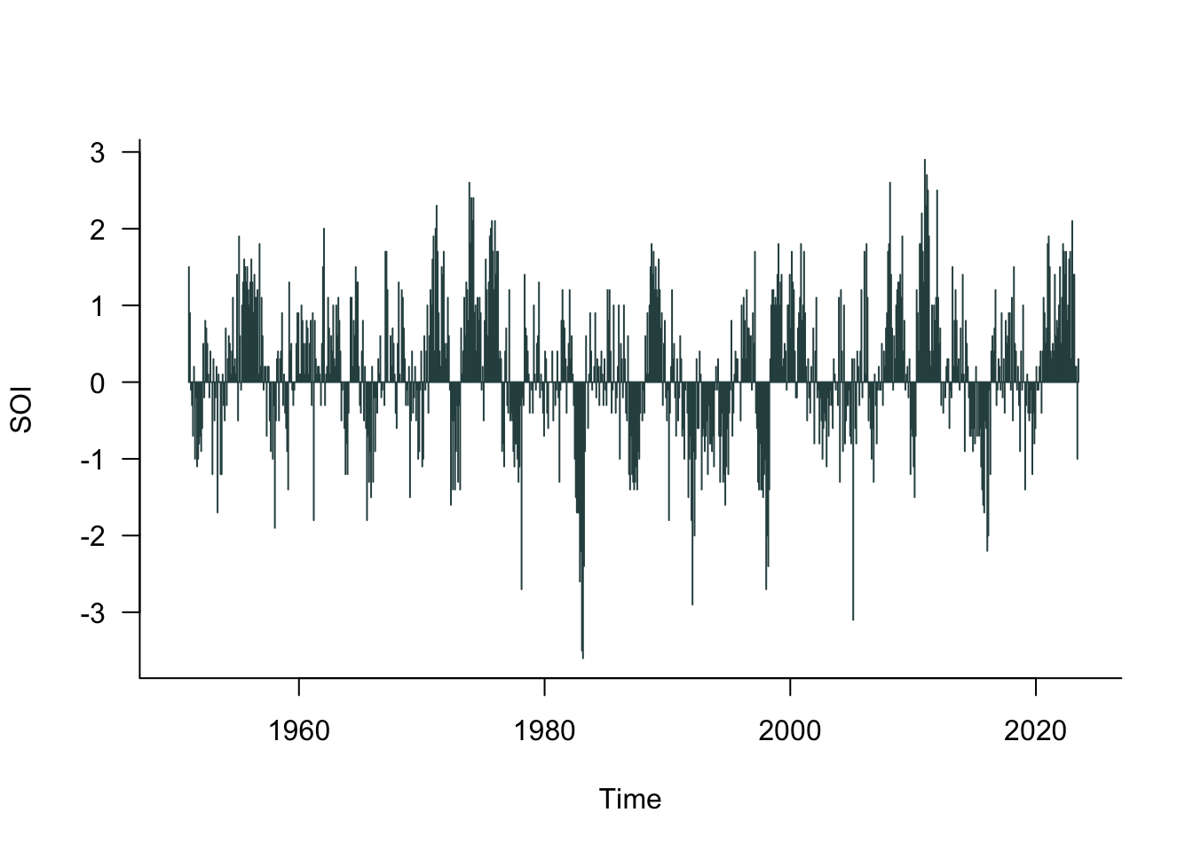
The Southern Oscillation Index (SOI) is a standardized index based on the observed sea level pressure differences between Tahiti and Darwin, Australia. The SOI is one measure of the large-scale fluctuations in air pressure occurring between the western and eastern tropical Pacific (i.e., the state of the Southern Oscillation) during El Niño and La Niña episodes.

In general, smoothed time series of the SOI correlate highly with changes in ocean temperatures across the eastern tropical Pacific. The negative phase of the SOI represents below-normal air pressure at Tahiti and above-normal air pressure at Darwin. Prolonged periods of negative (positive) SOI values coincide with abnormally warm (cold) ocean waters across the eastern tropical Pacific typical of El Niño (La Niña) episodes (Figure 31.1).

According to Wikipedia, there have been about 30 El Niño episodes since 1950 with strong El Niño events in 1982–83, 1997–98, and 2014–16. You recognize El Niño when the SOI dips negative for a period of time. La Niña is marked by periods of positive SOI values.

Figure 31.1: Monthly SOI data from 1951 to mid-2023 according to NOAA.

What is the signal and the noise in these data?
Is it possible that there are multiple signals in these data, associated with different time horizons?

Types of Statistical Learning

Isolation Forest

In Section 16.5 an isolation forest was used to identify outliers in a data set.

Describe why this is an unsupervised learning technique.
Describe how a supervised learning method for outlier detection would work.

Regression and Classification

Random Multiple-choice Answers

Suppose you administer a multiple-choice exam to a group of students who choose their answers completely at random.

The students with the top 10% of the scores are asked to take the exam a second time. Again, they answer the multiple-choice questions at random.

What percentage of the questions will the students taking the second exam get correct?
How does this relate to the regression to the mean phenomenon?

The Email Filter Detective

You have built an email spam detection model for your company. After testing it on 1,000 emails, you need to evaluate its performance. The confusion matrix below displays the results of classifying the 1,000 test emails with your model.

	Predicted: Spam	Predicted: Not Spam	Total
Actually Spam	320	80	400
Actually Not Spam	45	555	600
Total	365	635	1000

Part 1: Metrics

Calculate all metrics in Table 23.3.

What percentage of emails did the model classify correctly?
Of all emails flagged as spam, what percentage were actually spam?
Of all actual spam emails, what percentage did the model catch?
Of all legitimate emails, what percentage were correctly identified?

Part 2: Business Impact Analysis

Answer these questions about the real-world implications:

What do the 80 emails represent? What’s the business impact of this error type?
What do the 45 emails represent? What’s the business impact of this error type?
Which error type (from questions 1-2) is worse for user experience? Why?
If you had to choose, would you prefer a model with higher precision or higher recall? Justify your choice.

Changing the Email Filter Detective

Return to the confusion matrix in the previous exercise. The confusion table is based on classifying email as spam if the model predicts a probability of spam of more than 0.5 (this is the Bayes classifier). It turns out that your boss is not happy with the results and gives you two options to improve the model:

Option A: Adjust the threshold to reduce false positives by 50%, but false negatives will increase by 30%

Option B: Adjust the threshold to reduce false negatives by 60%, but false positives will double

Calculate accuracy, precision, and recall for the new confusion matrix for each option
Which option would you choose and why?
What would you tell your boss about the trade-offs?

Prediction

Every Day Predictions

Give five examples where you make predictions on a daily basis or where you are the subject of another system’s predictions.

Which of these predictions are based on an algorithm (to your knowledge), which are based on experience or gut feeling?

70% Chance of Rain

Research what it means when a meteorologist states “there is a 70% chance of rain tomorrow”.

Algorithmic vs Data Modeling

Recall the discussion of algorithmic modeling and data modeling from the first module. Data modeling is based on a probabilistic data-generating mechanism. Algorithmic modeling does not build models on the foundation of stochastic processes that explain the data.

What is the fundamental difference between the two approaches with respect to predictions?

Interactions

Two Factor Interaction

You are analyzing a study with two qualitative factors, A and B. A has two levels and B has three levels.

Give a verbal interpretation of what is meant by “factors A and B interact” and “factors A and B do not interact”.
Produce a plot similar to Figure 23.9 that shows interaction and lack of interaction between the two factors.
Interactions can mask main effects. For example, when an AxB interaction is significant but the A and B main effects are not, we say that the interaction masks the main effects. Suppose now that A and B both have two levels. What does the interaction plot look like if the AxB interaction masks the main effects?

31.3 Correlation and Causation

Correlation Coefficient

Anscombe’s Quartet

Use the file anscombe.csv, it contains four data sets created by statistician Francis Anscombe. The data sets are identified as variable pairs \((x_1,y_1)\) through \((x_4,y_4)\).

For each pair produce a scatter plot between \(X\) and \(Y\) and calculate the following statistics:

\(\overline{x}, \overline{y}\)
\(s_x, s_y\), the standard deviations of \(X\) and \(Y\)
\(\widehat{\rho}_{xy}\), the Pearson correlation coefficient between \(X\) and \(Y\)
The slope and intercept of a linear regression of \(Y\) on \(X\).

What do you conclude based on the plots and the calculated statistics?

Categorical Data

Odds Ratio

Compute the odds ratio for the data in Table 23.4. What do you conclude about the independence of observed and predicted values?

Rater Agreement

Refer to the data on the agreement of two raters in Table 24.1.

Compute the Kappa statistic for these data.
The theoretical maximum value of \(\kappa=1\) requires that the row and column totals are identical. For any given table, the maximum achievable value of \(\kappa\) is \[ \kappa_{\text{max}} = \frac{-\pi_e + \sum_{i=1}^r\min\{\pi_{i.},\pi_{.j}\}}{1-\pi_e} \] Here, \(\pi_{i.}\) and \(\pi_{.j}\) are the row and column probabilities, respectively. Using estimates for these probabilities based on the observed data, what is \(\kappa_{\text{max}}\) in this case?

Establishing Causality

Confounding: 1854 Cholera Outbreak

In the case of the 1854 cholera outbreak (see Section 2.8.1), there could have been confounding factors that caused cholera incidences in the Broad Street area to be higher, whether the water was or was not the cause of the disease. Maybe the residents of that poorer neighborhood had a different diet that caused the disease. Maybe they had occupations that made it more likely to be exposed to a harmful agent. Maybe. Maybe. Maybe.

What other confounding factors can you think of that would mask, amplify, or suppress the incidence of cholera?

Why Do Old Men Have Big Ears?

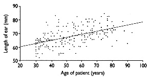
Spiegelhalter (2021, 108–9) asks the question “Why do old men have big ears?” based on his personal experience that older men seem to have big ears. This question cannot be answered with a randomized controlled trial, we cannot assign ear lengths. It is what it is.

Observational studies in the UK and Japan collected cross-sectional data, that is, a sample from the current population, which will include men of different ages. Analyzing the data the studies concluded that there is a positive correlation between age and ear length. For example, the figure below appeared in Heathcote (1995). The study concluded that the regression trend was significant. The slope of the regression line is 0.22mm per year with a 95% confidence interval of [0.17, 0.27] mm per year. Because the confidence interval does not cover the value 0, the trend is statistically significant. It seems that as we get older our ears get bigger by an average by 0.22 mm per year.

Try and explain the association between age and ear length in men. What are possible reasons ears are/appear larger in older men?
If you were to conduct a follow-up study to test the possible reasons in 1., what would the study look like? What kind of data would you collect? What kind of men would you recruit for the study?

Fluoride Exposure and IQ

The National Toxicology Program of the U.S. Department of Health and Human Services conducted a meta-analysis of the relationship between fluoride intake and IQ.

Among the findings of the analysis, the article states (emphasis in original):

The NTP monograph concluded, with moderate confidence, that higher levels of fluoride exposure, such as drinking water containing more than 1.5 milligrams of fluoride per liter, are associated with lower IQ in children. The NTP review was designed to evaluate total fluoride exposure from all sources and was not designed to evaluate the health effects of fluoridated drinking water alone. It is important to note that there were insufficient data to determine if the low fluoride level of 0.7 mg/L currently recommended for U.S. community water supplies has a negative effect on children’s IQ. The NTP found no evidence that fluoride exposure had adverse effects on adult cognition.

…

The determination about lower IQs in children was based primarily on epidemiology studies in non-U.S. countries such as Canada, China, India, Iran, Pakistan, and Mexico where some pregnant women, infants, and children received total fluoride exposure amounts higher than 1.5 mg fluoride/L of drinking water.

Read the full article from the National Toxicology Program here and answer the following questions:

Did the study establish correlation or causation between fluoride intake and children’s IQ?
Does the article make it clear whether to take the results as an indication of causation or correlation?
What is meta-analysis?
How do you interpret the fact that the study did not analyze data from the U.S.? Does that affect whether the results are applicable to U.S. children?
Can you think of confounding factors that limit transfer of the results to the U.S?
Are you surprised that there is no evidence of adverse effects on adults?

Link between Repeated Head Impacts and CTE

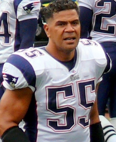
Tiaina Baul “Junior” Seau was an outstanding linebacker who played in the National Football League for 20 years, mostly with the San Diego Chargers and also the Miami Dolphins and New England Patriots. He committed suicide in 2012 by shooting himself in the chest. Junior did not leave a suicide note but a piece of paper with lyrics from the country song “Who I Ain’t”. An autopsy confirmed that Junior Seau had suffered from chronic traumatic encephalopahty (CTE) believed due to repeated head trauma he experienced as a football player.

Figure 31.3: Junior Seau playing for the New England Patriots. Source: Wikipedia

In July 2025, a gunman named Shane Tamura, walked into an office building in Manhattan and opened fire. The N.F.L. has an office in the building, and apparently, this is where he was headed. He took the wrong elevator and none of the four people he killed worked at the N.F.L. In his wallet he carried a note claiming that years of playing football had left him with CTE. After killing four people, Shane Tamura killed himself with a shot in the chest. The note said “Study my brain please.”

Nowinski et al. (2022) applied the Hill criteria to establish causality between repeated head impacts (RHI) and CTE. The authors discuss previous research on the association of the two and the resistance to calling the link between RHI and CTE causal. Interestingly, it appears that the causal link between the two was settled throughout the 20th century when causality was called into question again. The article is available online.

What reasons were given by some of the organizations involved in the debate (like CISG) to resist declaring a causal link between RHI and CTE?
What do you believe was their motivation to do so?
In the section Understanding Causation, the article examines each of Hill’s nine criteria. Cite one argument from the article in support of each criterion.
Per the Discussion section of the article, what are valid reasons why scientists might remain skeptical of a causal link between RHI and CTE?
What language did the authors use in the Conclusion to indicate a causal relationship between RHI and CTE?
Based on the evidence provided, should the conclusions drawn from data about adult athletes be applied to children? Argue for or against and why or why not?

31.4 Bias-Variance Tradeoff

The bias and variance of a model refer to the behavior of the model under conceptual repetitions of the sampling process. In Section 25.2 we simulated multiple sets of data and fit the models to each set.

In practice, we have only one set of data and need to infer bias and variance based on the single set. Bias and variance are then often associated with the flexibility of the model. You see statements such as “Flexible, wiggly models have a large variance; rigid (stiff) models have a large bias.”

The statement is not entirely incorrect, but I need you to explain to me in words how the connection is made between judging the flexibility of a model and the model behavior under conceptual repetition of sampling.

Mean Squared Error

Suppose that \(Y\) is a random variable with density function \[ f(y) = \frac{1}{\theta} \, e^{-y/\theta}\qquad \text{for } y > 0 \] The mean and variance of \(Y\) are \(\text{E}[Y] = \theta\) and \(\text{Var}[Y] = \theta^2\). You draw a random sample of size \(n=3\). Consider the following estimators of \(\theta\):

\(\widehat{\theta}_1 = Y_1\)
\(\widehat{\theta}_2 = \frac{Y1+Y2}{2}\)
\(\widehat{\theta}_3 = \frac{Y1+2Y2}{3}\)
\(\widehat{\theta}_4 = \overline{Y}\)

Calculate the mean square errors of the four estimators. Which estimator has the smallest MSE? Are any of the estimators biased?

Mean Squared Error

Return to the Anscombe data sets from the earlier assignment in this chapter. Compute the estimated mean squared error (\(\widehat{\text{MSE}}\)) on the training data for the four linear regression models.

31.5 Cross-validation

\(K\)-fold Cross-validation for Decision Tree

The following Python code generates a data set with 1000 observations, a target variable y and four input variables. The mean function is non-linear with local interactions, a situation where decision trees work well.

import numpy as np
import pandas as pd

# Set random seed for reproducibility
np.random.seed(42)

def generate_regression_dataset(n_samples=1000):
    """
    Generate a synthetic dataset for regression with multiple features
    that have non-linear relationships (good for decision trees)
    """
    # Generate features
    X1 = np.random.uniform(-5, 5, n_samples)  # Feature 1
    X2 = np.random.uniform(-3, 3, n_samples)  # Feature 2
    X3 = np.random.uniform(0, 10, n_samples)  # Feature 3
    X4 = np.random.normal(0, 1, n_samples)    # Feature 4
    
    # Create non-linear target variable with interactions
    # This type of relationship is well-suited for decision trees
    y = (2 * X1**2 + 
         np.where(X2 > 0, 3 * X2, -2 * X2) +  # Piecewise linear
         np.sin(X3) * 5 +                      # Sinusoidal
         X1 * X2 +                             # Interaction term
         X4 * 0.5 +                            # Linear component
         np.random.normal(0, 1, n_samples))    # Noise
    
    # Combine features into matrix
    X = np.column_stack([X1, X2, X3, X4])
    
    # Create feature names
    feature_names = ['x1_quadratic', 'x2_piecewise', 'x3_sinusoidal', 'x4_linear']
    
    return X, y, feature_names

# Generate the dataset
print("Generating synthetic regression dataset...")

Generating synthetic regression dataset...

X, y, feature_names = generate_regression_dataset(n_samples=1000)

print(f"\nDataset Info:")


Dataset Info:

print(f"  Features: {feature_names}")

  Features: ['x1_quadratic', 'x2_piecewise', 'x3_sinusoidal', 'x4_linear']

print(f"  Shape: {X.shape}")

  Shape: (1000, 4)

print(f"  Target range: [{y.min():.2f}, {y.max():.2f}]")

  Target range: [-4.63, 72.73]

The next code chunk fits a decision tree using a 75:25 train:test split and computes two metrics on the test data set: the R-square equivalent coefficient of determination and the mean square prediction error \(\widehat{MSE}_{\text{Test}}\). This code chunk should be helpful for the remainder of the assignment if you are not familiar with decision trees in Python.

from sklearn.tree import DecisionTreeRegressor
from sklearn.metrics import mean_squared_error, r2_score
from sklearn.model_selection import train_test_split

X_train, X_test, y_train, y_test = train_test_split(
    X, y, train_size=0.75, random_state=235)
            
model = DecisionTreeRegressor(
    max_depth=6,
    min_samples_split=10,
    min_samples_leaf=5
    )
            
# Train model
model.fit(X_train, y_train)

DecisionTreeRegressor(max_depth=6, min_samples_leaf=5, min_samples_split=10)

In a Jupyter environment, please rerun this cell to show the HTML representation or trust the notebook.
On GitHub, the HTML representation is unable to render, please try loading this page with nbviewer.org.

y_pred = model.predict(X_test)
            
# Calculate metrics
r2 = r2_score(y_test, y_pred)
mse = mean_squared_error(y_test, y_pred)
print(f"  R2 score: {r2:.3f}")

  R2 score: 0.902

print(f"  MSE_Test: {mse:.3f}")

  MSE_Test: 27.973

Task

Write a function that performs \(k\)-fold cross-validation and calculates across all folds the following:

Mean squared error for the test set.
Coefficient of determination (\(R^2\))

Report the min, max, mean, and standard deviation for these two statistics for \(k=5\), \(k=10\).

Plot the MSE and \(R^2\) values for the two values of \(k\).

Leave-One-Out Cross-validation for Decision Tree

How do you adjust the code in the previous assignment to perform leave-one-out cross-validation?

Perform the LOO CV and compare the result to the previous ones.
How much slower is the LOOCV compared to \(k\)-fold CW with \(k=5\) and \(k=10\)?

Compare with sklearn’s cross_val_score

Repeat the \(5\)-fold cross-validation exercise but now use cross_val_score in sklearn. How do the cross-validated mean squared error and \(R^2\) compare to the code you rolled yourself?